2.3 Arithmetic & Indexing
: 40 minutes
Now that we know how to create new tensors or NumPy arrays, let us talk about some of the vectorized operations we can perform on them.
Arithmetic Operations
Any arithmetic operations between equal-size arrays apply the operation element-wise as show below:
Arithmetic operations with scalars is also element-wise:
Array of equal size can also be compared element-wise. The output is a boolean array of same size.
Basic Indexing
We use indexing for viewing a subset of a NumPy array. NumPy indexing can be an extremely involved topic. For this course, we touch upon only some of the basic indexing techniques.
The most basic indexing resembles indexing of a Python list.
The above can also be used to edit an array, by populating the selected subset by a scalar.
Although array indexing works similarly, unlike Python lists, NumPy array slices are only views or perspectives on the original array. Consequently, mutating a slice propagates the same the mutation onto the original array.
In case you want a genuine copy of an array (or its slice), use numpy.copy().
For higher dimensional arrays or tensors, we need supply nested (equivalently comma-separated) index arguments to access individual data elements.
Advanced Indexing
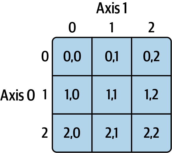
In order to understand more advanced indexing, we will need a thorough understanding of axis.
A matrix is a two dimensional tensor, and it has two axes. For convenience, you can think of the first axis (axis=0) as the rows, and the first axis (axis=1) along the columns. Although for tensors in general, it’s best not use the terms rows and columns to avoid any confusion. However, we can still use the axes.
For a multidimensional array A with k many axes, A[1] reveals (the view) of an array with (k-1) axes.
Since it’s just the view, scalar values and arrays can be assigned to A[1] to modify the portion of A.
Similarly, more indices can be used along other axes to further expose different parts of the array. The following returns a vector containing values whose indices start with 1 and end with 2.
Imagine the first axis (axis=0) being a collection of two (5, 2) matrices, namely A[0] and A[1] so that A[1, :, 2] returns the third column (axis=2) of the matrix A[1].
Indexing with Slices
Basic slicing for one-dimensional arrays works similar to Python lists. The only difference, again, is it’s only a view. Hence, changing the view mutates the original array.
Slicing a multi-dimensional array becomes a bit different. The following example slices an array along the first axis (axis=0), selecting the (2, 3)-sized matrices contained within the range 1:4.
You can mix and match integer indexing and slicing. A few examples below.
Boolean Indexing
A conditional statement can also be passed to select a subset of an array that satisfies the condition. When compared an array in a conditional statement, the (vectorized) comparison is element-wise, returning a boolean array.
This boolean array can now be passed to select a subset of any array.
Negate a statement using ~ and combine two statements using operators like & and |. Python kewords such as and and or don’t work as expected for NumPy.
Transposing Arrays and Swapping Axes
For a matrix \bold{A} of size (m, n), the transpose \bold{A}^T switches its rows and columns to form a matrix of size (n,m).
In NumPy the function .T does the trick. Once again, A.T returns only a view without altering the array A.
The higher-dimensional analog of transpose is swapping axes. For a NumPy array, any two axes can be swapped by using swapaxes(.,.). For a matrix A, it has the same effect as transpose:
More generally, any two axes can be chosen to be swapped.
In NumPy, .T is a special of axis swap to reverse all axes.