viewof v1 = Inputs.range([15, 85], {value: 25, step: 1, label: `age`})
viewof v2 = Inputs.range([50, 75], {value: 55, step: 1, label: `height`})
viewof v3 = Inputs.range([130, 250], {value: 170, step: 1, label: `weight`})
result = 3 * v1 + 5 * v2 - 2 * v3 > 100 ? "Male" : "Female"
result1 = 2 * v1 + 4.5 * v2 - 1.5 * v3 > 100 ? "Male" : "Female"8.1 Classical Machine Learning
: 45 minutes
A well-established definition of machine learning or ML due to Mitchell (1997) is the following:
Mitchell, T. M. 1997. Machine Learning. McGraw-Hill International Editions. McGraw-Hill.
A computer program is said to learn from experience \mathcal{E} with respect to some class of tasks \mathcal{T}, and performance measure \mathcal{P}, if its performance at tasks in \mathcal{T}, as measured by \mathcal{P}, improves with experience \mathcal{E}.
Depending on the task at hand, machine learning can be broadly classified into two main types: predictive or supervised and descriptive or unsupervised.

Supervised
In this regime of learning, we assume that there is a set \mathcal{X} containing all possible inputs \bold{x} and a set \mathcal{Y} containing all possible outputs y. And, there is an unknown mapping or rule f\colon\mathcal{X}\to\mathcal{Y} (unknown to us), which output an element y\in\mathcal{Y} given an input \bold{x}\in\mathcal{X}. The set of inputs, outputs, and the hidden rule depend on the task at hand.
The objective is to learn (or guess) the mapping—given a training dataset \mathcal{D}=\{(\bold{x}_i, y_i)\}_{i=1}^N containing N many labeled input-output pairs from the true mapping f. In other words, the motivation is to conjure up a guess mapping \widehat{f}:\mathcal{X}\to\mathcal{Y}.
In most applications, the inputs \bold{x}\in\mathbb{R}^d, i.e., a dimensional feature vector (x_1, x_2, \ldots, x_d) containing d scalars. Features are also called attributes or covariates. And, the output is called the response.
TipAn Example Mapping
Let us assume that there is a (god) mapping f that assigns the sex of a person given their age in [15,85] years, height in [50, 75] inch, and weight in [130, 250] lbs. The actual nature of f is hidden from us humans but we are only allowed to see the output for any input.
The features are age, height, and weight. So, the inputs \bold{x}\in\mathbb{R}^3.
In this example, the set of all possible inputs \mathcal{X}=[15, 85]\times[50, 75]\times[130, 250] and the set of outputs \mathcal{Y}=\{\textcolor{magenta}{Male}, \textcolor{green}{Female}\}.
An approximate mapping \widehat{f} is given below.
In applications, the features \bold{x} can be a very complicated object—such as images, point-clouds, molecular shapes, etc; the response can also often have more than just two labels.
Nonetheless, If the response is categorical, the learning problem is called classification or pattern recognition. When it is real-valued, the problem is known as regression.
Classification
A classification task involves predicting a qualitative (categorical) outcome, such as assigning a label or class to an observation. For instance, predicting whether an email is spam or not, or diagnosing a patient as having a specific type of cancer. Typically, the output set \mathcal{Y} consists of C unordered, discrete classes or labels \{1, 2, \ldots, C\}. In particular, when \mathcal{Y}=\{0, 1\} or \{-1, +1\} or \{Male, Female\}, it’s called a binary classification problem. When C>2, the problem is called multiclass classification.
Let’s take some real-world applications.
Iris Flowers
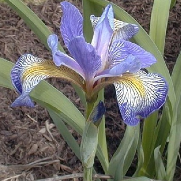
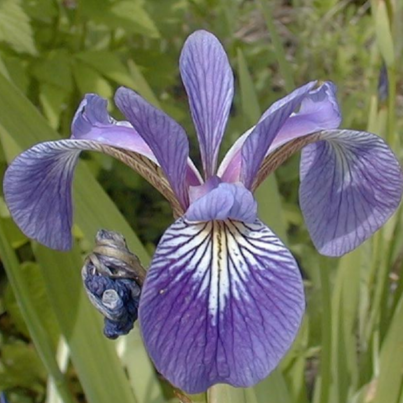
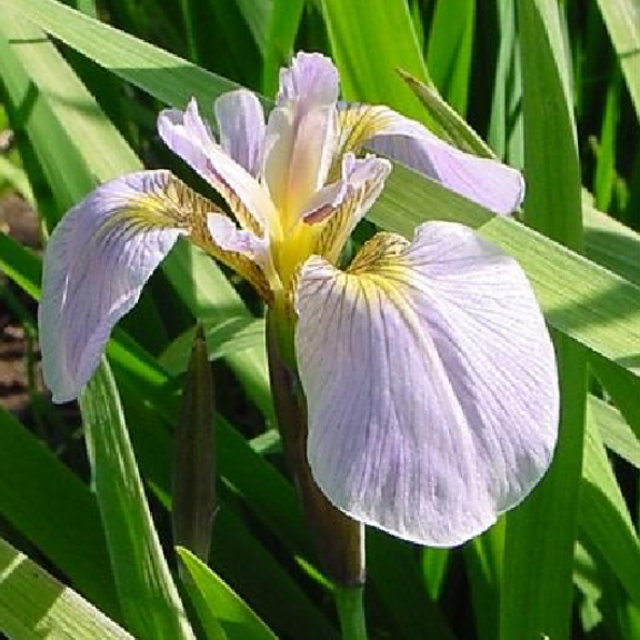
The famous Iris dataset was made famous in 1936 by the father of statistics: Ronald Fisher. The data consist of 50 samples from each of three species of Iris (Iris setosa, Iris versicolor and Iris virginica).
Murphy, Kevin P. 2012. Machine Learning: A Probabilistic Perspective. The MIT Press.
Four features were measured from each sample: the length and the width of the sepals and petals, in centimeters. We have already seen in class the distribution of the features across the subspecies; see Figure 24.2.
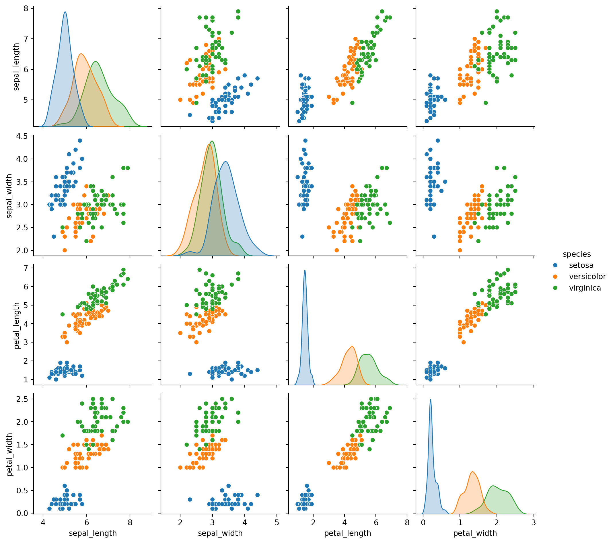
One can consider the problem of classifying Iris flowers into their 3 subspecies. In this case, the feature vector is four dimensional, \bold{x}\in\mathbb{R}^4 and \mathcal{Y}=\{Setosa, Versicolor, Virginica\} containing C=3 labels. Ronald Fisher used a linear discriminant analysis to approach the classification problem.
In practice, classifying images is an extremely challenging task— largely due the uncertainties around the choice of the features. In case of Iris, however, the botanists made the choice very easy for us identifying the four crucial features.
Digit Classification
In the Iris classification problem, the features were already identified by botanists. A much harder classification problem is to directly classify an image of handwritten digit. An example application is to recognize isolated handwritten digits in a ZIP code on a letter. The standard dataset used for this purpose is known as MNIST (Modified National Institute of Standards).
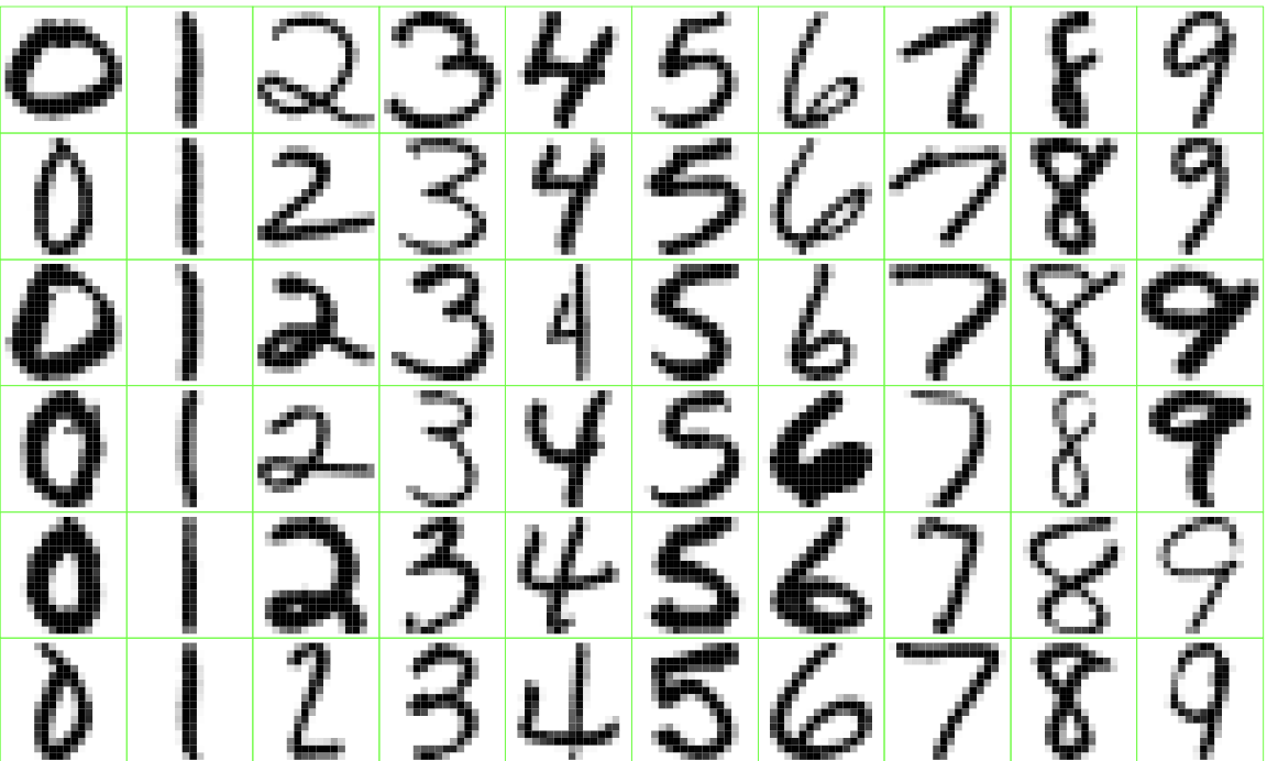
This dataset contains 60,000 training images and 10,000 test images of the digits 0 to 9, as written by various people. The images are size 28\times28 and have grayscale values in the range \{0, \ldots, 255\}. See Figure 24.3 for some examples.
Our input space \mathcal{X} is set of all 28\times28 matrices, also denoted by \mathbb{R}^{28\times28} and output space \mathcal{Y}=\{0, 1, 2, 3, 4, 5, 6, 7, 8, 9\}.
Regression
A regression task involves predicting a quantitative (numerical or continuous) outcome y\in\mathcal{Y} based on one or more input variables \bold{x}\in\mathcal{X}. Examples include:
Predict income from their age, years of eduction, tenure, experience
Predict the age of a viewer watching a given video on YouTube
Predict tomorrow’s stock given the historical stock data
Prostate Cancer
The prostate cancer data for this example come from a clinical study done in 1989, examining the correlation between the level of Prostate Specific Antigen (PSA) and a number of clinical measurements in 97 patients. Here, the goal is to predict the (log of) PSA (lpsa) from features including log cancer volume (lcavol), log prostate weight (lweight), age, log of benign prostatic hyperplasia amount (lbph), seminal vesicle invasion (svi), log of capsular penetration (lcp), Gleason score (gleason), and percent of Gleason scores 4 or 5 (pgg45). See Figure 24.4.

Unsupervised Learning
In unsupervised learning, for each observation i = 1, \dots, N, we observe a vector of features \bold{x}_i, but there is no associated response y_i. The objective in this setting, is to “make sense” of data instead of learning a mapping. This makes the task more challenging, as the goal is to uncover hidden structure or patterns in the data. Nonetheless, unsupervised learning allows us to learn models of “how the world works”, as Geoff Hinton said in :
When we’re learning to see, nobody’s telling us what the right answers are — we just look. Every so often, your mother says “that’s a dog”, but that’s very little information. You’d be lucky if you got a few bits of information — even one bit per second — that way. The brain’s visual system has \mathcal{O}(10^{14}) neural connections. And you only live for \mathcal{O}(10^9) seconds. So it’s no use learning one bit per second. You need more like \mathcal{O}(10^5) bits per second. And there’s only one place you can get that much information: from the input itself.
TipReinforcement Learning
There is also a third category called Reinforcement Learning (RL), which is beyond the scope of this class (though it is taught in the GWU Data Science program). Reinforcement learning is concerned with learning from trial and error to make decisions over time.
Unlike traditional types of learning, RL involves learning how to act in uncertain environments where outcomes are delayed and depend on sequences of actions. The goal is to learn an optimal policy for decision-making that maximizes cumulative reward.
Clustering
Clustering is an easy example of unsupervised learning. It involves identifying groups or clusters of similar observations without knowing any response labels. The goal is to discover structure in the data based only on the predictors. For instance, clustering might be used to segment customers by purchasing behavior, group articles by topic, or detect communities in a network.
The clustering algorithm groups observations so that those within the same cluster are more similar (according to some distance or similarity metric) than those in different clusters. For example, we present below the scatterplot pedal_width vs petal_length, ignoring the labels.
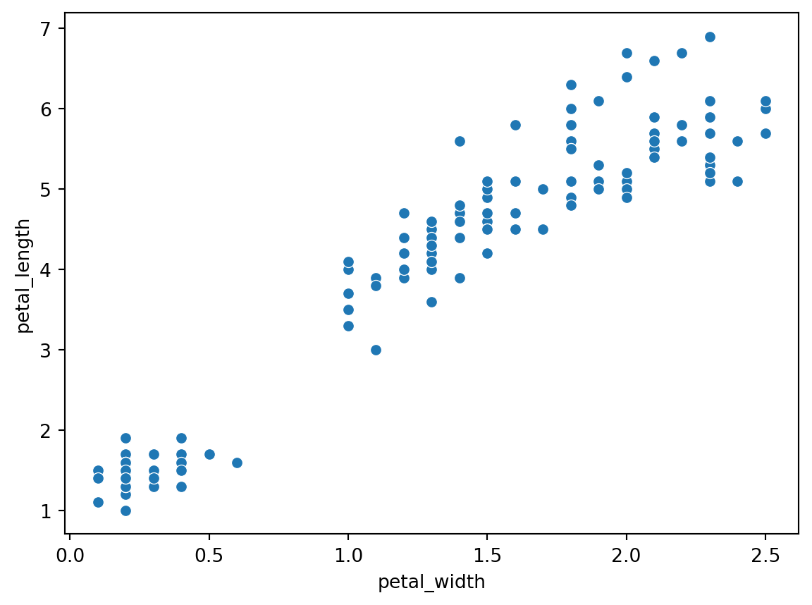
In Figure 24.5, we can clearly see two visually separated clusters. The lower left cluster, in fact, contains all samples from subspecies setosa; whereas, the other cluster in the top right corner contains the other two subspecies.
Dimensionality Reduction
Other examples of unsupervised learning includes dimensionality reduction: reducing the data dimension by projecting onto a much lower-dimensional space without losing much of the “essence” of the data. The Principal Component Analysis (PCA) captures low-dimensinal latent dimensions still trying to preserve the variation exists in the data. Manifold Learning, on the other hand, tries to learn a much lower-dimensional latent manifold.

Figure: Types of Tasks in Machine Learning