9.1 Binary Logistic Regression

: 120 minutes

The binary classification problem assumes that the output set \mathcal{Y} has two unordered, discrete labels or classes: \mathcal{Y}=\{\tt 0, \tt 1\}; and, the label of each sample is exactly one of them. Examples include predicting

• admission to an academic program based on standardized test scores,
• credit card default using their spending behavior,
• breast cancer diagnosis, etc.

We use Binary Logistic Regression (a.k.a., Sigmoid Regression) to solve the binary classification problem.

Recall that there are d predictors or features (x_1, x_2, \ldots, x_d). For notational convenience with weights, we preppend 1 to the vector when denoting our feature vector, i.e., \bold{x}=(1, x_1, x_2, \ldots, x_d) is a (d+1)-vector.

In case d=1, the problem is called univariate, otherwise multivariate.

Model Assumptions

We always assume that the underlying rule f is unknowable to us, much like a “blackbox”. In binary logistic regression, we make two model assumptions about the blackbox:

1. the conditional probability p(y\mid \bold{x}) follows a Bernoulli distribution¹ with mean \mu(\bold{x});

2. the conditional mean \mu(\bold{x}) is the sigmoid² of a linear function of \bold{x}, i.e., \mu(\bold{x})=\frac{1}{1+e^{-(\bold{x}\bold{w}^T)}}.

¹ A random variable Z with two outputs \{\tt 0, 1\} is said to follow a Bernoulli distribution with mean \mu\in[0,1] if its probability density function: p(z)=\begin{cases}\mu,&\text{ if } z={\tt 1}\\ 1-\mu,&\text{ if }z={\tt 0} \end{cases}

² the sigmoid (S-shaped) function is denoted by \mathrm{sigm}(t)\colon\mathbb{R}\to\mathbb{R}. It maps the entire real line to the interval [0,1]; see Figure 26.1

The (d+1) weights w_0, w_1, \ldots, w_d are the parameters \pmb{\theta} of the model. Since the number of parameters does not grow with the size of the data, this is a parametric model.

function sigmoid(x, k=1, x0=0) {
  return 1 / (1 + Math.exp(-k * (x - x0)));
}
data = {
  const points = [];
  for (let x = -10; x <= 10; x += 0.1) {
    points.push({ x: x, y: sigmoid(x, 1, 0) });
  }
  return points;
}

Plot.plot({
  width: 700,
  height: 400,
  marginLeft: 60,
  marginBottom: 60,
  grid: true,
  x: {
    label: "t →",
    domain: [-10, 10]
  },
  y: {
    label: "↑ sigm(t)",
    domain: [0, 1]
  },
  marks: [
    Plot.line(data, {
      x: "x",
      y: "y",
      stroke: "#349a32ff",
      strokeWidth: 3
    }),
    Plot.ruleY([0.5], { 
      stroke: "#94a3b8", 
      strokeDasharray: "4,4",
      strokeWidth: 1
    }),
    Plot.ruleX([0], { 
      stroke: "#94a3b8", 
      strokeDasharray: "4,4",
      strokeWidth: 1
    })
  ]
});

Figure 26.1

Since, we are making a model assumption in terms of the conditional probability for the first time in this course, it deserves an explanation. Feel free to digress to a motivating example before continuing.

Mathematical Formulation

We now describe the mathematical formulation for the multivariate case with d\geq1 predictors x_1, x_2, \ldots, x_d. The key components are the following:

• Feature vector: \bold{x}=(1, x_1, \ldots, x_d)
• Binary output: y={\tt 0}\text{ or }{\tt 1}
• Model weights: \bold{w}=(w_0, w_1, \ldots, w_d)
• w_0 is called the bias or intercept

As per our model assumption, we have p({\tt 1}\mid\bold{x}; \bold{w})= \frac{1}{1+e^{-(\bold{x}\bold{w}^T)}} =\frac{1}{1+e^{-(w_0+w_1x_1+\ldots+w_dx_d)}} \tag{26.1}

Learning and Prediction

Given a dataset \mathcal{D}=\{(\bold{x}_i, y_i)\}_{i=1}^N of size N from the blackbox f, we learn an approximation \hat{f} by learning the weights \bold{w}.

Here, each (boldfaced) input \bold{x}_i represents a vector (1, x_{i1}, x_{i2}, \ldots, x_{id}) and corresponding output y_i is either \tt 1 or \tt 0.

If \bold{w}^*=(w_0^*, w_1^*, \ldots, w_d^*) denotes our learned weights, we can write from Equation 26.1 our learned class probability for y=\tt 1: \hat{p}({\tt 1}\mid \bold{x};\bold{w}^*) =\frac{1}{1+e^{-(w^*_0+w^*_1x_1+\ldots+w^*_dx_d)}} \tag{26.2}

Using Equation 26.2, we can then predict the label or class of new data point with feature vector \bold{x} using a threshold function. For example, the following classifier uses a threshold of 0.5: \hat{y}=\begin{cases} {\tt 1}&\text{ if }\hat{p}({\tt 1}\mid\bold{x};\bold{w}^*)\geq0.5 \\ {\tt 0}&\text{ if }\hat{p}({\tt 1}\mid\bold{x};\bold{w}^*)<0.5. \end{cases} \tag{26.3}

Loss Function and Optimization

Now, we turn our attention to finding the best or optimal weights, w.r.t. some notion of loss or error. We use the Maximum Likelihood Estimator (a.k.a. MLE) to maximize the odds or probability of the occurrence of the given data \mathcal{D} across all choices of the weights.

Since the data is i.i.d., the likelihood of the dataset \mathcal{D} is given by: p(\mathcal{D}; \bold{w})\coloneqq \prod_{i=1}^N p(y_i\mid \bold{x}_i; \bold{w}).

Using the above model assumptions, we can write the likelihood as: p(\mathcal{D}; \bold{w}) =\prod_{i=1}^N p({\tt 1}\mid\bold{x}_i)^{y_i}[1-p({\tt 1}\mid\bold{x}_i)]^{1-y_i}. The log likelihood \mathrm{LL}(\bold{w}) as: \begin{aligned} \log{p(\mathcal{D}; \bold{w})} &=\log{\left(\prod_{i=1}^N p({\tt 1}\mid\bold{x}_i)^{y_i}[1-p({\tt 1}\mid\bold{x}_i)]^{1-y_i}\right)} \\ &=\sum_{i=1}^N \log{\left(p({\tt 1}\mid\bold{x}_i)^{y_i}[1-p({\tt 1}\mid\bold{x}_i)]^{1-y_i}\right)} \\ &=\sum_{i=1}^N y_i\log{p({\tt 1}\mid\bold{x}_i)}+(1-y_i)\log{[1-p({\tt 1}\mid\bold{x}_i)]}. \end{aligned}

Finally, the loss function \bold{\mathcal L}(\bold{w}), known as Average Binomial Cross Entropy, is given by the average negative log likelihood: \bold{\mathcal L}(\bold{w}) \coloneqq-\frac{1}{N}\sum_{i=1}^N y_i\log{p({\tt 1}\mid\bold{x}_i)}+(1-y_i)\log{[1-p({\tt 1}\mid\bold{x}_i)]}, \tag{26.4} where p({\tt 1}\mid \bold{x};\bold{w}) is as assumed in Equation 26.1.

Minimizing \bold{\mathcal L}(\bold{w}) across all possible weights \pmb{w}\in\mathbb{R}^(d+1) to find the optimal weight \pmb{w}^* is a computationally challenging problem. One would traditionally use the Gradient Descent to solve the optimization problem.

We will use scikit-learn in this course. Once the optimal weights have been found, Equation 26.3 can be used to propose a classifier.

Metrics for Classification

In regression, we used metrics like the Mean Squared Error (MSE) and \mathcal{R}^2 as metrics for “good of fit”. In classification, we use a different set of metrics:

• Confusion Matrix
• (Overall) Accuracy
• (Class-specific) Precision, Recall, and F1-score

Confusion Matrix

In binary classification problem, the confusion matrix is a 2\times2 matrix that captures to what degree a classifier misclassifies the (training/test) data.

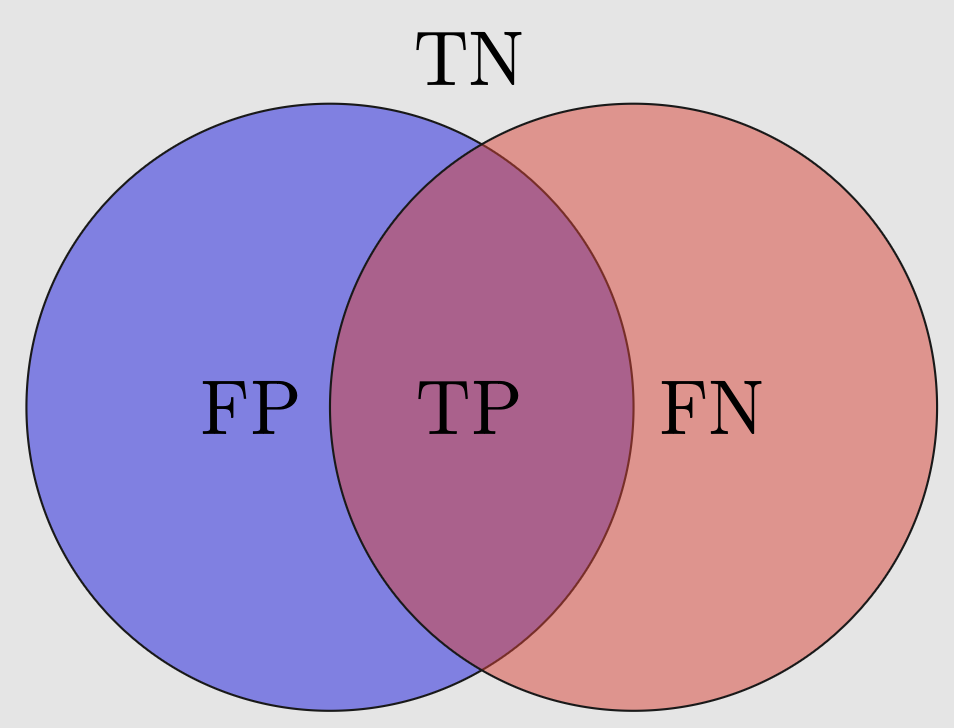
Using the convention that \tt 1=POSITIVE and \tt 0=NEGATIVE, we define:

• \text{\color{green}True Positive} (TP): an observation is classified by the classifier as POSITIVE while its original label was POSITIVE, as desired;
• \text{\color{green}True Negative} (TN): an observation is classified by the classifier as NEGATIVE while its original label is NEGATIVE, as desired;
• \text{\color{red}False Positive} (FP): an observation is (mis)classified by the classifier as POSITIVE while its original label is NEGATIVE;
• \text{\color{red}False Negative} (FN): an observation is (mis)classified by the classifier as NEGATIVE while its original label was POSITIVE;

Since the above cases are exhaustive, we have the following Venn diagram:

The Venn Diagram

Figure 26.2

A yet better representation scheme is reporting the number of observations that fall into the above four cases as a matrix: the confusion matrix:

{
  const width = 500;
  const height = 500;
  const margin = 120;
  
  const svg = d3.create("svg")
    .attr("viewBox", `0 0 ${width} ${height}`)
    .attr("width", width)
    .attr("height", height);
  
  const boxSize = (width - 2 * margin) / 2;
  
  // Title
  svg.append("text")
    .attr("x", width / 2)
    .attr("y", 50)
    .attr("text-anchor", "middle")
    .attr("font-size", "35px")
    .text("Predicted Class");
  
  // Predicted labels (top)
  svg.append("text")
    .attr("x", margin + boxSize / 2)
    .attr("y", 110)
    .attr("text-anchor", "middle")
    .attr("font-size", "30px")
    .html("P̂");
  
  svg.append("text")
    .attr("x", margin + boxSize * 1.5)
    .attr("y", 110)
    .attr("text-anchor", "middle")
    .attr("font-size", "30px")
    .html("N̂");
  
  // Actual Class label (left, rotated)
  svg.append("text")
    .attr("x", -height / 2)
    .attr("y", 35)
    .attr("text-anchor", "middle")
    .attr("font-size", "35px")
    .attr("transform", `rotate(-90)`)
    .text("Actual Class");
  
  // Actual labels (left)
  svg.append("text")
    .attr("x", 85)
    .attr("y", margin + boxSize / 2 + 10)
    .attr("text-anchor", "middle")
    .attr("font-size", "30px")
    .text("P");
  
  svg.append("text")
    .attr("x", 85)
    .attr("y", margin + boxSize * 1.5 + 10)
    .attr("text-anchor", "middle")
    .attr("font-size", "30px")
    .text("N");
  
  // Boxes
  const boxes = [
    { x: 0, y: 0, label: ["True", "Positive", "(TP)"] },
    { x: 1, y: 0, label: ["False", "Negative", "(FN)"] },
    { x: 0, y: 1, label: ["False", "Positive", "(FP)"] },
    { x: 1, y: 1, label: ["True", "Negative", "(TN)"] }
  ];
  
  boxes.forEach(box => {
    const g = svg.append("g");
    
    // Rectangle
    g.append("rect")
      .attr("x", margin + box.x * boxSize)
      .attr("y", margin + box.y * boxSize)
      .attr("width", boxSize)
      .attr("height", boxSize)
      .attr("fill", "none")
      .attr("stroke", "gray")
      .attr("stroke-width", 2);
    
    // Text
    const textX = margin + box.x * boxSize + boxSize / 2;
    const baseY = margin + box.y * boxSize + boxSize / 2 - 30;
    
    box.label.forEach((line, i) => {
      g.append("text")
        .attr("x", textX)
        .attr("y", baseY + i * 40)
        .attr("text-anchor", "middle")
        .attr("font-size", "30px")
        .text(line);
    });
  });
  
  return svg.node();
}

Figure 26.3: The Confusion Matrix

It’s evident from Figure 26.3 above that \begin{aligned} P &= TP + FN\\ N &= FP + TN\\ \hat P &=TP + FP\\ \hat N &=TN + FN. \end{aligned}

TipAccuracy

The accuracy measures the rate of the correct classification: acc = \frac{TP+TN}{TP+TN+FP+FN} \tag{26.5}

For imbalanced data, it’s recommended to class-specific precision as a more robust performance metric for a classifier.

TipPrecision

The precision of a class measures the rate of the correct classification among labels classified as the class: p_{\tt 1} = \frac{TP}{TP+FP}\text{ and } p_{\tt 0} = \frac{TN}{TN+FN}. \tag{26.6}

TipRecall

The recall of a class measures the rate of the correct classification among true labels in that class: r_{\tt 1} = \frac{TP}{TP+FN}\text{ and } r_{\tt 0} = \frac{TN}{TN+FP} \tag{26.7}

Note Precision vs Recall

Compute the accuracy of a model that renders the following confusion matrix: \begin{bmatrix} 22 & 10 \\ 5 & 25 \end{bmatrix}.

\bold{y}=\frac{1}{d}(\bold{z}-c\bold{x})\bold{y}=\frac{1}{d}(\bold{z}+c\bold{x})\bold{y}=\frac{\bold{z}-c\bold{x}}{d}Not always possible

Possible only when d\neq0. In that case, we can write \bold{y}=\frac{1}{d}(\bold{z}-c\bold{x}).

TipF1-score

The F1 score of the positive and negative classes are defined, respectively, as follows: f_{\tt 1} = \frac{2p_{\tt 1}r_{\tt 1}}{p_{\tt 1}+r_{\tt 1}}\text{ and } f_{\tt 0} = \frac{2p_{\tt 0}r_{\tt 0}}{p_{\tt 0}+r_{\tt 0}}. \tag{26.8}

Note Confusion Matrix

Compute the accuracy of a model that renders the following confusion matrix: \begin{bmatrix} 22 & 10 \\ 5 & 25 \end{bmatrix}.

\bold{y}=\frac{1}{d}(\bold{z}-c\bold{x})\bold{y}=\frac{1}{d}(\bold{z}+c\bold{x})\bold{y}=\frac{\bold{z}-c\bold{x}}{d}Not always possible

Possible only when d\neq0. In that case, we can write \bold{y}=\frac{1}{d}(\bold{z}-c\bold{x}).

A Motivating Example

Let us consider a practical binary classification problem with just one predictor. We ask how GW offers admission to a student? In order to keep our example simple, we base our analysis around just one predictor: SAT scores.

In our analysis, the only feature x is SAT score in the range [400, 1600], and the output y\in\{{\tt 0},{\tt 1}\} with \tt 1=Admission offered and \tt 0=Not offered.

As always, the rule or mapping f that GW applies to decide the output is assumed to be unknowable. Nonetheless, we can always give f a nudge to give us i.i.d. data for training.

The Data

Choose N below to get a sample \mathcal{D}=\{(x_i, y_i)\}_{i=1}^N:

rnd = d3.randomInt(400, 1600);
D = d3.range(N).map(() => {
      const x = rnd()
      const y = d3.randomBernoulli(sigmoid(w0+w1 * x))();
      return {x: x, y: y} 
});
P = D.map( (e) => {
      return {...e, phat: sigmoid(w0_opt+w1_opt * e.x), yhat: sigmoid(w0_opt+w1_opt * e.x) >= thres ? 1 : 0} 
});
L = function(D, w0, w1) {
  return D.reduce( (res, e) =>
    res - [e.y * Math.log(sigmoid(w0+w1*e.x)) + (1-e.y) * Math.log(1-sigmoid(w0+w1*e.x))], 0
  ) / D.length;
}
viewof N = Inputs.range([0, 100], {value: 20, step: 1, label: tex`N`})

Let take a look at our \mathcal{D}:

Inputs.table(D, {
  columns: [
    "x",
    "y"
  ],
  header: {
    x: "SAT Score",
    y: "Admission"
  }
})

Let’s also plot the data:

Plot.plot({
  x: {label: '(x) SAT Score'},
  y: {label: '(y) Admission'},
  grid: true,
  marks: [
    Plot.dot(D, {
      x: "x", 
      y: "y",
      fill: (d) => d.y == 1 ? "green" : "red",
      opacity: 0.7
    })
  ]
})

viewof w0 = Inputs.range([-50, 50], {value: -4.7, step: 0.1, label: tex`w_0`})
viewof w1 = Inputs.range([0, 1], {value: 0.005, step: .001, label: tex`w_1`})

Logistic Regression

We now decide to use logistic regression to develop our own classifier that will hopefully approximate GW’s mysterious admission rule f with high accuracy.

In logistic regression, we have two model assumptions. The mathematical formulation of the assumptions is already presented. Here, we plainly discuss what the assumptions mean this our context.

Let us assume that that insider told you that instead of a holistic assessment, GW uses the following naive rule f to offer admission, solely based on an applicant’s SAT score x.

1. the rule first takes a weighted SAT of the applicant x\mapsto w_0+w_1x

2. then Sigmoid is applied on the weighted score to make it a positive fraction w_0+w_1x\mapsto\mathrm{sigm}(w_0+w_1x)

3. finally, a coin with probability of HEADS equals \mathrm{sigm}(w_0+w_1x) is tossed.

4. the applicant is offered admission if the outcome from the toss render HEADS, otherwise not.

The only critical information your insider did not have access to were the weights w_0 and w_1!

Guessing the Solution

Recall that the loss \bold{\mathcal{L}}(\mathcal{D}; w_0, w_1) as given in Equation 26.4 can be computed for any weights w_0, w_1 of your choice.

We can bruteforce the optimization by plotting the incurred loss for a variety of choices for the weights. In the following surface represents the loss:

Plotly = require("https://cdn.plot.ly/plotly-latest.min.js")
// Import Plotly from CDN
a = {
  const n = 200;
  return d3.range(-20, 20, 40/n);
}
b = {
  const n = 300;
  return d3.range(-0.02, 0.02, 0.04/n);
}
surfaceData = {
  const z = [];
  for (let i = 0; i < b.length; i++) {
    const row = [];
    for (let j = 0; j < a.length; j++) {
      row.push(L(D, a[j], b[i]));
    }
    z.push(row);
  }
  
  return [{
    type: 'surface',
    showscale: false,
    x: a,
    y: b,
    z: z,
    colorscale: 'Greens',
    contours: {
      z: {
        show: true,
        usecolormap: true,
        highlightcolor: "red",
        project: { z: true }
      }
    }
  }];
}

// Create the plot
{
  const div = DOM.element('div');
  Plotly.newPlot(div, surfaceData, {
    title: 'Cross-entropy',
    scene: {
      xaxis: { title: "w_0" },
      yaxis: { title: "w_1" },
      zaxis: { title: "L" },
      camera: {
        eye: { x: 1.5, y: 1.5, z: 1.3 }
      },
    },
    width: "100%",
    height: 700
  });
  
  return div;
}

Your Classifier

Find the mininum.

viewof w0_opt = Inputs.number({value: -4.7, label: tex`w_0^*`})
viewof w1_opt = Inputs.number({value: 0.005, label: tex`w_1^*`})
data_pred = {
  const points = [];
  for (let x = 400; x <= 1600; x += 1) {
    points.push({ x: x, y: sigmoid(w0_opt+w1_opt*x, 1, 0) });
  }
  return points;
}
x_thres = -(w0_opt+Math.log(1/thres-1))/w1_opt
Plot.plot({
  grid: true,
  marks: [
    Plot.line(d3.range(400, x_thres).map(x => ({x, y: 0})), {
      x: "x", 
      y: "y", 
      stroke: "red",
      opacity: 0.3, 
      strokeWidth: 3
    }),
    Plot.line(d3.range(x_thres, 1600).map(x => ({x, y: 0})), {
      x: "x", 
      y: "y", 
      stroke: "green",
      opacity: 0.3, 
      strokeWidth: 3
    }),
    Plot.dot(D, {
      x: "x", 
      y: "y",
      fill:  (d) => d.y == 1 ? "green" : "red",
      opacity: 0.7
    }),
    Plot.line(data_pred, {
      x: "x",
      y: "y",
      stroke: "#1a4987ff",
      opacity: 0.6,
      strokeWidth: 2
    })
  ]
})

viewof thres = Inputs.range([0.1, 0.9], {value: 0.5, step: 0.1, label: 'Threshold'})

Confusion Matrix:

{
  const width = 500;
  const height = 500;
  const margin = 120;
  const tp = P.filter((e) => e.y == 1 && e.yhat == 1).length;
  const fn = P.filter((e) => e.y == 1 && e.yhat == 0).length;
  const fp = P.filter((e) => e.y == 0 && e.yhat == 1).length;
  const tn = P.filter((e) => e.y == 0 && e.yhat == 0).length;
  const svg = d3.create("svg")
    .attr("viewBox", `0 0 ${width} ${height}`)
    .attr("width", width)
    .attr("height", height);
  
  const boxSize = (width - 2 * margin) / 3;
  
  // Title
  svg.append("text")
    .attr("x", width / 2)
    .attr("y", 50)
    .attr("text-anchor", "middle")
    .attr("font-size", "35px")
    .text("Predicted Class");
  
  // Predicted labels (top)
  svg.append("text")
    .attr("x", margin + boxSize / 2)
    .attr("y", 110)
    .attr("text-anchor", "middle")
    .attr("font-size", "25px")
    .html("P̂");
  
  svg.append("text")
    .attr("x", margin + boxSize * 1.5)
    .attr("y", 110)
    .attr("text-anchor", "middle")
    .attr("font-size", "25px")
    .html("N̂");
  
  svg.append("text")
    .attr("x", margin + boxSize * 2.5)
    .attr("y", 110)
    .attr("text-anchor", "middle")
    .attr("font-size", "25px")
    .html("Rec.");
  
  // Actual Class label (left, rotated)
  svg.append("text")
    .attr("x", -height / 2)
    .attr("y", 35)
    .attr("text-anchor", "middle")
    .attr("font-size", "35px")
    .attr("transform", `rotate(-90)`)
    .text("Actual Class");
  
  // Actual labels (left)
  svg.append("text")
    .attr("x", 85)
    .attr("y", margin + boxSize / 2 + 10)
    .attr("text-anchor", "middle")
    .attr("font-size", "30px")
    .text("P");
  
  svg.append("text")
    .attr("x", 85)
    .attr("y", margin + boxSize * 1.5 + 10)
    .attr("text-anchor", "middle")
    .attr("font-size", "30px")
    .text("N");
  
  svg.append("text")
    .attr("x", 85)
    .attr("y", margin + boxSize * 2.5 + 10)
    .attr("text-anchor", "middle")
    .attr("font-size", "25px")
    .text("Prec.");

  // Boxes
  const boxes = [
    { x: 0, y: 0, label: ["(TP)", tp] },
    { x: 1, y: 0, label: ["(FN)", fn] },
    { x: 2, y: 0, label: [`(r_1)`, parseFloat(tp/(tp+fn)).toFixed(2)] },
    { x: 0, y: 1, label: ["(FP)", fp] },
    { x: 1, y: 1, label: ["(TN)", tn] },
    { x: 2, y: 1, label: [`(r_0)`, parseFloat(tn/(fp+tn)).toFixed(2)] },
    { x: 0, y: 2, label: [`(p_1)`, parseFloat(tp/(tp+fp)).toFixed(2)] },
    { x: 1, y: 2, label: [`(p_0)`, parseFloat(tn/(fn+tn)).toFixed(2)] },
    { x: 2, y: 2, label: ["Acc", parseFloat((tp+tn)/(tp+fn+fp+tn)).toFixed(2)] },
  ];
  
  boxes.forEach(box => {
    const g = svg.append("g");
    
    // Rectangle
    g.append("rect")
      .attr("x", margin + box.x * boxSize)
      .attr("y", margin + box.y * boxSize)
      .attr("width", boxSize)
      .attr("height", boxSize)
      .attr("fill", "none")
      .attr("stroke", "gray")
      .attr("stroke-width", 2);
    
    // Text
    const textX = margin + box.x * boxSize + boxSize / 2;
    const baseY = margin + box.y * boxSize + boxSize / 2 - 18;
    
    box.label.forEach((line, i) => {
      g.append("text")
        .attr("x", textX)
        .attr("y", baseY + i * 40)
        .attr("text-anchor", "middle")
        .attr("font-size", "25px")
        .text(line);
    });
  });
  
  return svg.node();
}

Figure 26.4: The Confusion Matrix