compute_c = function (points) {
  return points.y1 - compute_m(points) * points.x1;
}
compute_m = function (points) {
  return (points.y1 - points.y2) / (points.x1 - points.x2);
}
update = function (svg, X, Y, zrange, strech, sep) {
  const xdomain = X.domain();
  const ydomain = Y.domain();
  const m = compute_m(pivots);
  const c = compute_c(pivots);

  svg
    .select("#line")
    .attr("stroke", sep ? "black" : "lightgray")
    .attr(
      "x1",
      m * xdomain[0] + c >= ydomain[0] ? X(xdomain[0]) : X((ydomain[0] - c) / m)
    )
    .attr(
      "y1",
      m * xdomain[0] + c >= ydomain[0] ? Y(m * xdomain[0] + c) : Y(ydomain[0])
    )
    .attr(
      "x2",
      m * xdomain[1] + c >= ydomain[0] ? X(xdomain[1]) : X((ydomain[0] - c) / m)
    )
    .attr(
      "y2",
      m * xdomain[1] + c >= ydomain[0] ? Y(m * xdomain[1] + c) : Y(ydomain[0])
    );

  svg
    .select("#R1")
    .attr(
      "points",
      [
        [X(xdomain[0]), Y(m * xdomain[0] + c)],
        [X(xdomain[1]), Y(m * xdomain[1] + c)],
        [X(xdomain[1]), Y(m * xdomain[1] + c + strech)],
        [X(xdomain[0]), Y(m * xdomain[0] + c + strech)]
      ].join(",")
    )
    .style("fill", zrange[0])
    .style("opacity", 0.1);
  svg
    .select("#R2")
    .attr(
      "points",
      [
        [X(xdomain[0]), Y(m * xdomain[0] + c)],
        [X(xdomain[1]), Y(m * xdomain[1] + c)],
        [X(xdomain[1]), Y(m * xdomain[1] + c - strech)],
        [X(xdomain[0]), Y(m * xdomain[0] + c - strech)]
      ].join(",")
    )
    .style("fill", zrange[1])
    .style("opacity", 0.1);

  svg
    .select("#M1")
    .attr(
      "points",
      [
        [X(xdomain[0]), Y(m * xdomain[0] + c)],
        [X(xdomain[1]), Y(m * xdomain[1] + c)],
        [X(xdomain[1]), Y(m * xdomain[1] + c + margin * Math.sqrt(1 + m * m))],
        [X(xdomain[0]), Y(m * xdomain[0] + c + margin * Math.sqrt(1 + m * m))]
      ].join(",")
    )
    .style("fill", zrange[0])
    .style("opacity", 0.3);

  svg
    .select("#M2")
    .attr(
      "points",
      [
        [X(xdomain[0]), Y(m * xdomain[0] + c)],
        [X(xdomain[1]), Y(m * xdomain[1] + c)],
        [X(xdomain[1]), Y(m * xdomain[1] + c - margin * Math.sqrt(1 + m * m))],
        [X(xdomain[0]), Y(m * xdomain[0] + c - margin * Math.sqrt(1 + m * m))]
      ].join(",")
    )
    .style("fill", zrange[1])
    .style("opacity", 0.3);
}
separates = function (data, x, y, z) {
  const m = compute_m(pivots);
  const c = compute_c(pivots);
  if (data[0][y] > m * data[0][x] + c)
    return data.every(
      (d) =>
        (d[z] == data[0][z] && d[y] > m * d[x] + c) ||
        (d[z] != data[0][z] && d[y] < m * d[x] + c)
    );
  else if (data[0][y] < m * data[0][x] + c)
    return data.every(
      (d) =>
        (d[z] == data[0][z] && d[y] < m * d[x] + c) ||
        (d[z] != data[0][z] && d[y] > m * d[x] + c)
    );
  else return false;
}
draw = function (data, args = {}) {
  // Declare the chart dimensions and margins.
  const width = args.width || 600;
  const height = args.width || 400;
  const marginTop = args.marginTop || 5;
  const marginRight = args.marginRight || 20;
  const marginBottom = args.marginBottom || 50;
  const marginLeft = args.marginLeft || 40;
  const x = args.x || "x";
  const y = args.y || "y";
  const z = args.z || "z";
  const xdomain = args.xdomain || [0, d3.max(data, (d) => d[x])];
  const ydomain = args.ydomain || [0, d3.max(data, (d) => d[y])];
  const zdomain = args.zdomain || [0, 1];
  const zrange = args.zrange || ["red", "blue"];
  const m = compute_m(pivots);
  const c = compute_c(pivots);

  // Declare the x (horizontal position) scale.
  const X = d3
    .scaleLinear()
    .domain(xdomain)
    .range([marginLeft, width - marginRight]);

  // Declare the y (vertical position) scale.
  const Y = d3
    .scaleLinear()
    .domain(ydomain)
    .range([height - marginBottom, marginTop]);

  // Declare the fill axis
  const Z = d3.scaleOrdinal().domain(zdomain).range(zrange);

  // Create the SVG container.
  const svg = d3.create("svg").attr("width", width).attr("height", height);

  // Add the x-axis.
  svg
    .append("g")
    .attr("transform", `translate(0,${height - marginBottom})`)
    .call(d3.axisBottom(X));
  svg.append("text")
    .attr("text-anchor", "end")
    .attr("x", width - 50)
    .attr("y", height - 20 )
    .text("age (x1) →");
  svg.append("text")
    .attr("text-anchor", "end")
    .attr("transform", "rotate(-90)")
    .attr("y",  13)
    .attr("x", -20)
    .text("education (x2) →")

  // Add the y-axis.
  svg
    .append("g")
    .attr("transform", `translate(${marginLeft},0)`)
    .call(d3.axisLeft(Y));

  const regions = svg.append("g").attr("id", "regions");
  regions.append("polygon").attr("id", "R1");
  regions.append("polygon").attr("id", "R2");

  // Add the dots
  svg
    .append("g")
    .selectAll("dot")
    .data(data)
    .enter()
    .append("circle")
    .attr("cx", (d) => X(d[x]))
    .attr("cy", (d) => Y(d[y]))
    .attr("r", 3)
    .style("fill", (d) => Z(d[z]));

  // Show Margins
  svg.append("g").attr("id", "margins");
  regions.append("polygon").attr("id", "M1");
  regions.append("polygon").attr("id", "M2");

  // Add the line
  const line = svg.append("g");

  line
    .append("line")
    .attr("id", "line")
    .attr("stroke-width", 3)
    .attr("path-length", 10);

  update(svg, X, Y, zrange, Math.max(width, height), separates(data, x, y, z));

  // Draw the pivot points
  line
    .append("circle")
    .attr("cx", X(pivots.x1))
    .attr("cy", Y(pivots.y1))
    .attr("r", 7)
    .style("fill", "white")
    .style("stroke", "lightgrey")
    .style("stroke-width", 3)
    .call(
      d3.drag().on("drag", function (event, d) {
        pivots.x1 = X.invert(event.x);
        pivots.y1 = Y.invert(event.y);

        d3.select(this).attr("cx", X(pivots.x1)).attr("cy", Y(pivots.y1));
        update(
          svg,
          X,
          Y,
          zrange,
          Math.max(width, height),
          separates(data, x, y, z)
        );
      })
    );
  line
    .append("circle")
    .attr("cx", X(pivots.x2))
    .attr("cy", Y(pivots.y2))
    .attr("r", 7)
    .style("fill", "white")
    .style("stroke", "lightgrey")
    .style("stroke-width", 3)
    .call(
      d3.drag().on("drag", function (event, d) {
        pivots.x2 = X.invert(event.x);
        pivots.y2 = Y.invert(event.y);

        d3.select(this).attr("cx", X(pivots.x2)).attr("cy", Y(pivots.y2));
        update(
          svg,
          X,
          Y,
          zrange,
          Math.max(width, height),
          separates(data, x, y, z)
        );
      })
    );

  // Draw regions
  if (showRegions) {
    regions.attr("visibility", "visible");
    regions.attr("visibility", "visible");
  } else {
    regions.attr("visibility", "hidden");
    regions.attr("visibility", "hidden");
  }

  // Draw line
  if (showLine) {
    line.attr("visibility", "visible");
    line.attr("visibility", "visible");
  } else {
    line.attr("visibility", "hidden");
    line.attr("visibility", "hidden");
  }

  // Return the SVG element.
  return svg.node();
}
generateData = function (xmin = -1, xmax = 1, ymin = -1, ymax = 1, n = 10, method = "linear") {
  const randX = d3.randomUniform(xmin, xmax);
  const randY = d3.randomUniform(ymin, ymax);
  const pivots = {
    x1: randX(),
    x2: randX(),
    y1: randY(),
    y2: randY()
  };
  const a = d3.randomUniform(0, 20)();
  const b = d3.randomUniform(0, 10)();

  return d3.range(n).map((d) => {
    const x = randX();
    const y = randY();
    let z;
    if (method == "linear")
      z = y - compute_m(pivots) * x - compute_c(pivots) > 0 ? 0 : 1;
    else if (method == "quad") {
      z = (x - 50) * (x - 50) / (a * a) + (y - 8) * (y - 8) / (b * b) - 1 > 0 ? 0 : 1;
    }
    return {
      x: x,
      y: y,
      z: z
    };
  });
}
10.1 Kernel-based Learning
ImportantPrerequisites
Must-have:
Enthusiasm about ML
Basics of matrix operations
- Linear Algebra
- My summer course on Linear Algebra and Convex Optimization
Python (pandas, numpy, scikit-learn)
- DATS-6103
Recommended:
Introduction
As always, we ask the following questions as we encounter a new learning algorithm:
- Classification or regression?
- Classification—default is binary
- Supervised or unsupervised?
- Supervised—training data are labeled
- Parametric or non-parametric?
- Parametric—it assumes a hypothesis class, namely hyperplanes
A Motivating Example
Let us ask the curious question: can we learn to predict party affiliation of a US national from their age and years of education?
Number of features: n=2.
Feature space: \mathcal{X} is a subset of \mathbb{R}^2.
Target space: \mathcal{Y}={
RED,BLUE}.
In the demo, we are trying to:
separate the separate our training examples by a line.
once we have learned a separating line, an unseen test point can be classified based on which side of the hyperplane the point is.
TipSummary
In summary, the SVM tries to learn from a sample a linear decision boundary that fully separates the training data.
Pros
- Very intuitive
- Efficient algorithms are available
- Linear Programming Problem
- Perceptron (rosenblatt1958perceptron?)
- Easily generalized to a higher-dimensional feature space
- decision boundary: line (n=2), plane (n=3), hyperplane (n\geq3)
Cons
- There are infinitely many separating hyperplanes
- maximum-margin
- The data may not be always linearly separable
- soft-margin
- Kernel methods
The Separable Case (Hard-Margin)
Let’s assume that the data points are linearly separable. Out of the infinitely many separating lines, we find the one with the largest margin.
Mathematical Formulation
Feature Space:
\mathcal{X}\subset\mathbb{R}^n is an n-dimensional space.
feature vector \pmb{x} is an n\times 1 vector
Target Space:
- \mathcal{Y}=\{-1, 1\}
Training Sample:
size m
S=\{(\pmb{x_1},y_1),\ldots,(\pmb{x_m},y_m)\}
- each x_i\in\mathcal{X}
- each y_i\in\mathcal{Y}
I.I.D. (why?)
Objective
Find a hyperplane \pmb{w}\cdot\pmb{x}+b=0 such that
all sample points are on the correct side of the hyperplane, i.e., y_i(\pmb{\pmb{w}\cdot\pmb{x_i}}+b)\geq0\text{ for all }i\in[1,m]
the margin (distance to the closed sample point) \rho=\min_{i\in[1, m]}\frac{|\pmb{w}\cdot\pmb{x_i}+b|}{\|\pmb{w}\|} is maximum
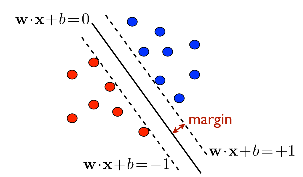
The good news is a unique solution hyperplane exists—so long as the sample points are linearly separable.
ImportantSolving the Optimization Problem
The primal problem can be stated as \min_{\pmb{w},b}\frac{1}{2}\|\pmb{w}\|^2 subject to: y_i(\pmb{w}\cdot\pmb{x_i}+b)\geq1\text{ for all }i\in[1,m] This is a convex optimization problem with a unique solution (\pmb{w}^*,b*).
Hence, the problem can be solved using quadratic programming (QP).
Moreover, the normal vector \pmb{w}^* is a linear combination of the training feature vectors: \pmb{w^*}=\alpha_1\pmb{x_1}+\ldots+\alpha_m\pmb{x_m}. If the i-th training vector appears in the above linear combination (i.e., \alpha_i\neq0), then it’s called a support vector.
TipDecision Rule
For an unseen test data-point with feature vector \pmb{x}, we classify using the following rule: \pmb{x}\mapsto\text{sign}(\pmb{w}^*\cdot\pmb{x}+b^*) =\text{sgn}\left(\sum_{i=1}^m\alpha_iy_i\pmb{x_i}\cdot\pmb{x}+b^*\right).
TipCode
The Non-Separable Case (Soft-Margin)
In real applications, the sample points are never separable. In that case, we allow for exceptions.
We would not mind a few exceptional sample points lying inside the maximum margin or even on the wrong side of the margin. However, the less number of exceptions, the better.
We toss a hyper-parameter C\geq0 (known as the regularization parameter) in to our optimization.
ImportantSolving with Slack Variables
The primal problem is to find a hyperplane (given by the normal vector \pmb{w}\in\mathbb{R}^n and b\in\mathbb{R}) so that \min_{\pmb{w},b,\pmb{\xi}}\left(\frac{1}{2}\|\pmb{w}\|^2 + C\sum_{i=1}^m\xi^2_i\right) subject to: y_i(\pmb{w}\cdot\pmb{x_i}+b)\geq1-\xi_i\text{ for all }i\in[m] Here, the \pmb{\xi}=(\xi_1,\ldots,\xi_m) is called the slack.
This is a also convex optimization problem with a unique solution.
However, in order to get the optimal solution, we consider the dual problem. For more details (foma?).
Consequently the objective of the optimization becomes two-fold:
maximize the margin
limit the total amount of slack.
TipCode
Choosing C
Some of the common choices are 0.001, 0.01, 0.1, 1.0, 100, etc. However, we usually use cross-validation to choose the best value for C.
TipCode
Non-Linear Boundary
For datasets, the inherit decision boundary is non-linear.
- Can our SVM be extended to handle such cases?
TipCode
Kernel Methods
A kernel K:\mathcal{X}\times\mathcal{X}\to\mathbb{R}^+ mimics the concept of inner-product, but for a more general Hilbert Space. Some of the good (for optimization) kernels are:
Linear Kernel: hyperplane separation or usual inner-product K(\pmb{x}, \pmb{x}')=\langle\pmb{x}, \pmb{x}'\rangle
Radial Basis Function (RBF): K(\pmb{x}, \pmb{x}')=\exp{\left(-\frac{\|\pmb{x}-\pmb{x}'\|^2}{2\sigma^2}\right)}.
TipCode
Digit Recognition using SVM
TipCode
Conclusion
Theoretically well-understood.
Extremely promising in applications.
Works well for balanced data. If not balanced:
- resample
- use class weights
Primarily a binary classifier. However, multi-class classification can be done using:
- one-vs-others
- one-vs-one
- Read more on Medium
Resources
- Books:
- Introduction to Statistical Learning, Chapter 9.
- Code:
- Hypothesis note-taking tool