10.2 Support Vector Machines

As always, we ask the following questions as we encounter a new learning algorithm:

Classification or regression?
- Classification—default is binary
Supervised or unsupervised?
- Supervised—training data are labeled
Parametric or non-parametric?
- Non-Parametric
  1. it does not make any assumption about the data
  2. the number of parameters not fixed across different datasets

A Motivating Example

Let us ask the curious question: can we learn to predict party affiliation of a US national from their age (x_1) and years of education (x_2)?

Number of features: n=2.
Feature space: \mathcal{X} is a subset of \mathbb{R}^2.
Target space: \mathcal{Y}={RED, BLUE}.

pivots = Object({ x1: 20, y1: 1, x2: 70, y2: 10 });
data = generateData(18, 80, 0, 15, 20, separable ? "linear" : "quad");
draw(
  data.map((d) => ({ x: d.x, y: d.y, z: d.z })),
  {
    x: "x",
    y: "y",
    xdomain: [18, 80],
    ydomain: [0, 15]
  }
);

viewof showLine = Inputs.toggle({ value: false, label: "Show line" });
viewof margin = Inputs.range([0, 5], {
  value: 0,
  step: 0.01,
  label: "Margin"
});
viewof showRegions = Inputs.toggle({ value: false, label: "Classified regions" });
viewof separable = Inputs.toggle({ value: true, label: "Separable?" });

Learning Objective

We are trying to:

separate our training examples by a line.
once we have learned a separating line, an unseen test point can be classified based on which side of the hyperplane the point is.

Summary

In summary, the SVM tries to learn from data a linear decision boundary that fully separates the training data.

Before we talk about the mathematical formulation, let us discuss the pros and cons.

Pros

Very intuitive
Efficient algorithms are available
- Linear Programming Problem
- Perceptron (Rosenblatt 1958)
Easily generalized to a higher-dimensional feature space
- decision boundary: line (n=2), plane (n=3), hyperplane (n\geq3)

Rosenblatt, F. 1958. “The perceptron: A probabilistic model for information storage and organization in the brain.” Psychological Review 65 (6): 386–408. https://doi.org/10.1037/h0042519.

Cons

There are infinitely many separating hyperplanes
- maximum-margin
The data may not be always linearly separable
- soft-margin
- Kernel methods

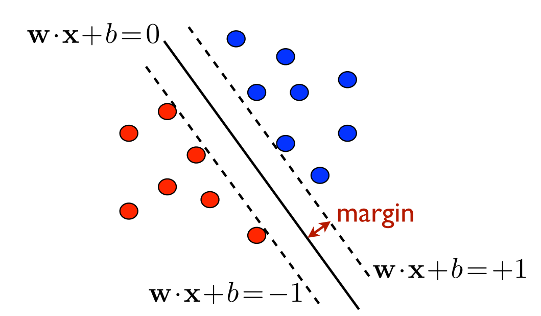
The Separable Case (Hard-Margin)

Let’s assume that the data points are linearly separable. Out of the infinitely many separating lines, we find the one with the largest margin.

Mathematical Formulation

Feature Space:

\mathcal{X}\subset\mathbb{R}^n is an n-dimensional space.
feature vector \pmb{x} is an n\times 1 vector

Target Space:

\mathcal{Y}=\{-1, 1\}

Training Data:

size N
\mathcal{D}=\{(\bold{x}_1,y_1),\ldots,(\bold{x}_N,y_N)\}
- each \bold{x}_i\in\mathcal{X}
- each y_i\in\mathcal{Y}

Objective

Find a hyperplane \langle\bold{w},\bold{x}\rangle+b=0. such that
all sample points are on the correct side of the hyperplane, i.e., y_i(\langle\bold{w},\bold{x_i}\rangle+b)\geq0\text{ for all }i=1,\ldots,N
the margin (distance to the closed sample point) \rho=\min_{i\in[1, N]}\frac{|\langle\bold{w},\bold{x_i}\rangle|+b}{\|\bold{w}\|} is maximum

The good news is a unique solution hyperplane exists—so long as the sample points are linearly separable.

Solving the Optimization Problem (optional)

The primal problem can be stated as \min_{\bold{w},b}\frac{1}{2}\|\bold{w}\|^2 subject to: y_i(\langle\bold{w},\bold{x_i}\rangle+b)\geq1\text{ for all }i\in[1,N] This is a convex optimization problem with a unique solution (\bold{w}^*,b^*).

Hence, the problem can be solved using quadratic programming (QP).

Moreover, the normal vector \pmb{w}^* is a linear combination of the training feature vectors: \bold{w^*}=\alpha_1\bold{x_1}+\ldots+\alpha_N\bold{x_N}. If the i-th training vector appears in the above linear combination (i.e., \alpha_i\neq0), then it’s called a support vector.

Decision Rule

For an unseen test data-point with feature vector \pmb{x}, we classify using the following rule: \bold{x}\mapsto\text{sign}(\langle\bold{w}^*,\bold{x}\rangle+b^*) =\text{sgn}\left(\sum_{i=1}^N\alpha_iy_i\langle\bold{x_i},\bold{x}\rangle+b^*\right).

The Non-Separable Case (Soft-Margin)

In real applications, the sample points are never separable. In that case, we allow for exceptions.

We would not mind a few exceptional sample points lying inside the maximum margin or even on the wrong side of the margin. However, the less number of exceptions, the better.

We toss a hyper-parameter C\geq0 (known as the regularization parameter) in to our optimization.

Solving with Slack Variables

The primal problem is to find a hyperplane (given by the normal vector \bold{w}\in\mathbb{R}^n and b\in\mathbb{R}) so that \min_{\bold{w},b,\bold{\xi}}\left(\frac{1}{2}\|\bold{w}\|^2 + C\sum_{i=1}^N\xi^2_i\right) subject to: y_i(\bold{w}\cdot\bold{x_i}+b)\geq1-\xi_i\text{ for all }i\in[N] Here, the \bold{\xi}=(\xi_1,\ldots,\xi_N) is called the slack.

This is a also convex optimization problem with a unique solution.

However, in order to get the optimal solution, we consider the dual problem. For more details (Mohri, Rostamizadeh, and Talwalkar 2018, chap. 5).

Mohri, Mehryar, Afshin Rostamizadeh, and Ameet Talwalkar. 2018. Foundations of Machine Learning. 2nd ed. The MIT Press.

Consequently the objective of the optimization becomes two-fold:

maximize the margin
limit the total amount of slack.

viewof C = Inputs.range([0, 100], {label: 'C', step: 0.001, value: 0.001})

Choosing C

Some of the common choices are 0.001, 0.01, 0.1, 1.0, 100, etc. However, we usually use cross-validation to choose the best value for C.

Non-Linear Boundary

For datasets, the inherit decision boundary is non-linear.

Can our SVM be extended to handle such cases?

Kernel Methods

A kernel K:\mathcal{X}\times\mathcal{X}\to\mathbb{R}^+ mimics the concept of inner-product, but for a more general Hilbert Space. Some of the good (for optimization) kernels are:

Linear Kernel: hyperplane separation or usual inner-product \mathcal K(\bold{x}, \bold{x}')=\langle\bold{x}, \bold{x}'\rangle
Radial Basis Function (RBF): \mathcal K(\bold{x}, \bold{x}')=\exp{\left(-\frac{\|\bold{x}-\bold{x}'\|^2}{2\sigma^2}\right)}.

Digit Recognition using SVM

Conclusion

Theoretically well-understood.
Extremely promising in applications.
Works well for balanced data. If not balanced:
- resample
- use class weights
Primarily a binary classifier. However, multi-class classification can be done using:
- one-vs-others
- one-vs-one
- Read more on Medium

Resources

Books:
- Introduction to Statistical Learning, Chapter 9.
Code:
- svm.zip

References

compute_c = function (points) {
  return points.y1 - compute_m(points) * points.x1;
}
compute_m = function (points) {
  return (points.y1 - points.y2) / (points.x1 - points.x2);
}
update = function (svg, X, Y, zrange, strech, sep) {
  const xdomain = X.domain();
  const ydomain = Y.domain();
  const m = compute_m(pivots);
  const c = compute_c(pivots);

  svg
    .select("#line")
    .attr("stroke", sep ? "black" : "lightgray")
    .attr(
      "x1",
      m * xdomain[0] + c >= ydomain[0] ? X(xdomain[0]) : X((ydomain[0] - c) / m)
    )
    .attr(
      "y1",
      m * xdomain[0] + c >= ydomain[0] ? Y(m * xdomain[0] + c) : Y(ydomain[0])
    )
    .attr(
      "x2",
      m * xdomain[1] + c >= ydomain[0] ? X(xdomain[1]) : X((ydomain[0] - c) / m)
    )
    .attr(
      "y2",
      m * xdomain[1] + c >= ydomain[0] ? Y(m * xdomain[1] + c) : Y(ydomain[0])
    );

  svg
    .select("#R1")
    .attr(
      "points",
      [
        [X(xdomain[0]), Y(m * xdomain[0] + c)],
        [X(xdomain[1]), Y(m * xdomain[1] + c)],
        [X(xdomain[1]), Y(m * xdomain[1] + c + strech)],
        [X(xdomain[0]), Y(m * xdomain[0] + c + strech)]
      ].join(",")
    )
    .style("fill", zrange[0])
    .style("opacity", 0.1);
  svg
    .select("#R2")
    .attr(
      "points",
      [
        [X(xdomain[0]), Y(m * xdomain[0] + c)],
        [X(xdomain[1]), Y(m * xdomain[1] + c)],
        [X(xdomain[1]), Y(m * xdomain[1] + c - strech)],
        [X(xdomain[0]), Y(m * xdomain[0] + c - strech)]
      ].join(",")
    )
    .style("fill", zrange[1])
    .style("opacity", 0.1);

  svg
    .select("#M1")
    .attr(
      "points",
      [
        [X(xdomain[0]), Y(m * xdomain[0] + c)],
        [X(xdomain[1]), Y(m * xdomain[1] + c)],
        [X(xdomain[1]), Y(m * xdomain[1] + c + margin * Math.sqrt(1 + m * m))],
        [X(xdomain[0]), Y(m * xdomain[0] + c + margin * Math.sqrt(1 + m * m))]
      ].join(",")
    )
    .style("fill", zrange[0])
    .style("opacity", 0.3);

  svg
    .select("#M2")
    .attr(
      "points",
      [
        [X(xdomain[0]), Y(m * xdomain[0] + c)],
        [X(xdomain[1]), Y(m * xdomain[1] + c)],
        [X(xdomain[1]), Y(m * xdomain[1] + c - margin * Math.sqrt(1 + m * m))],
        [X(xdomain[0]), Y(m * xdomain[0] + c - margin * Math.sqrt(1 + m * m))]
      ].join(",")
    )
    .style("fill", zrange[1])
    .style("opacity", 0.3);
}
separates = function (data, x, y, z) {
  const m = compute_m(pivots);
  const c = compute_c(pivots);
  if (data[0][y] > m * data[0][x] + c)
    return data.every(
      (d) =>
        (d[z] == data[0][z] && d[y] > m * d[x] + c) ||
        (d[z] != data[0][z] && d[y] < m * d[x] + c)
    );
  else if (data[0][y] < m * data[0][x] + c)
    return data.every(
      (d) =>
        (d[z] == data[0][z] && d[y] < m * d[x] + c) ||
        (d[z] != data[0][z] && d[y] > m * d[x] + c)
    );
  else return false;
}
draw = function (data, args = {}) {
  // Declare the chart dimensions and margins.
  const width = args.width || 600;
  const height = args.width || 400;
  const marginTop = args.marginTop || 5;
  const marginRight = args.marginRight || 20;
  const marginBottom = args.marginBottom || 50;
  const marginLeft = args.marginLeft || 40;
  const x = args.x || "x";
  const y = args.y || "y";
  const z = args.z || "z";
  const xdomain = args.xdomain || [0, d3.max(data, (d) => d[x])];
  const ydomain = args.ydomain || [0, d3.max(data, (d) => d[y])];
  const zdomain = args.zdomain || [0, 1];
  const zrange = args.zrange || ["red", "blue"];
  const m = compute_m(pivots);
  const c = compute_c(pivots);

  // Declare the x (horizontal position) scale.
  const X = d3
    .scaleLinear()
    .domain(xdomain)
    .range([marginLeft, width - marginRight]);

  // Declare the y (vertical position) scale.
  const Y = d3
    .scaleLinear()
    .domain(ydomain)
    .range([height - marginBottom, marginTop]);

  // Declare the fill axis
  const Z = d3.scaleOrdinal().domain(zdomain).range(zrange);

  // Create the SVG container.
  const svg = d3.create("svg").attr("width", width).attr("height", height);

  // Add the x-axis.
  svg
    .append("g")
    .attr("transform", `translate(0,${height - marginBottom})`)
    .call(d3.axisBottom(X));
  svg.append("text")
    .attr("text-anchor", "end")
    .attr("x", width - 50)
    .attr("y", height - 20 )
    .text("age (x1) →");
  svg.append("text")
    .attr("text-anchor", "end")
    .attr("transform", "rotate(-90)")
    .attr("y",  13)
    .attr("x", -20)
    .text("education (x2) →")

  // Add the y-axis.
  svg
    .append("g")
    .attr("transform", `translate(${marginLeft},0)`)
    .call(d3.axisLeft(Y));

  const regions = svg.append("g").attr("id", "regions");
  regions.append("polygon").attr("id", "R1");
  regions.append("polygon").attr("id", "R2");

  // Add the dots
  svg
    .append("g")
    .selectAll("dot")
    .data(data)
    .enter()
    .append("circle")
    .attr("cx", (d) => X(d[x]))
    .attr("cy", (d) => Y(d[y]))
    .attr("r", 3)
    .style("fill", (d) => Z(d[z]));

  // Show Margins
  svg.append("g").attr("id", "margins");
  regions.append("polygon").attr("id", "M1");
  regions.append("polygon").attr("id", "M2");

  // Add the line
  const line = svg.append("g");

  line
    .append("line")
    .attr("id", "line")
    .attr("stroke-width", 3)
    .attr("path-length", 10);

  update(svg, X, Y, zrange, Math.max(width, height), separates(data, x, y, z));

  // Draw the pivot points
  line
    .append("circle")
    .attr("cx", X(pivots.x1))
    .attr("cy", Y(pivots.y1))
    .attr("r", 7)
    .style("fill", "white")
    .style("stroke", "lightgrey")
    .style("stroke-width", 3)
    .call(
      d3.drag().on("drag", function (event, d) {
        pivots.x1 = X.invert(event.x);
        pivots.y1 = Y.invert(event.y);

        d3.select(this).attr("cx", X(pivots.x1)).attr("cy", Y(pivots.y1));
        update(
          svg,
          X,
          Y,
          zrange,
          Math.max(width, height),
          separates(data, x, y, z)
        );
      })
    );
  line
    .append("circle")
    .attr("cx", X(pivots.x2))
    .attr("cy", Y(pivots.y2))
    .attr("r", 7)
    .style("fill", "white")
    .style("stroke", "lightgrey")
    .style("stroke-width", 3)
    .call(
      d3.drag().on("drag", function (event, d) {
        pivots.x2 = X.invert(event.x);
        pivots.y2 = Y.invert(event.y);

        d3.select(this).attr("cx", X(pivots.x2)).attr("cy", Y(pivots.y2));
        update(
          svg,
          X,
          Y,
          zrange,
          Math.max(width, height),
          separates(data, x, y, z)
        );
      })
    );

  // Draw regions
  if (showRegions) {
    regions.attr("visibility", "visible");
    regions.attr("visibility", "visible");
  } else {
    regions.attr("visibility", "hidden");
    regions.attr("visibility", "hidden");
  }

  // Draw line
  if (showLine) {
    line.attr("visibility", "visible");
    line.attr("visibility", "visible");
  } else {
    line.attr("visibility", "hidden");
    line.attr("visibility", "hidden");
  }

  // Return the SVG element.
  return svg.node();
}
generateData = function (xmin = -1, xmax = 1, ymin = -1, ymax = 1, n = 10, method = "linear") {
  const randX = d3.randomUniform(xmin, xmax);
  const randY = d3.randomUniform(ymin, ymax);
  const pivots = {
    x1: randX(),
    x2: randX(),
    y1: randY(),
    y2: randY()
  };
  const a = d3.randomUniform(0, 20)();
  const b = d3.randomUniform(0, 10)();

  return d3.range(n).map((d) => {
    const x = randX();
    const y = randY();
    let z;
    if (method == "linear")
      z = y - compute_m(pivots) * x - compute_c(pivots) > 0 ? 0 : 1;
    else if (method == "quad") {
      z = (x - 50) * (x - 50) / (a * a) + (y - 8) * (y - 8) / (b * b) - 1 > 0 ? 0 : 1;
    }
    return {
      x: x,
      y: y,
      z: z
    };
  });
}