3.1 Multi-Armed Bandit Framework
We saw from Lecture 1 that Reinforcement Learning is about sequential decision-making:
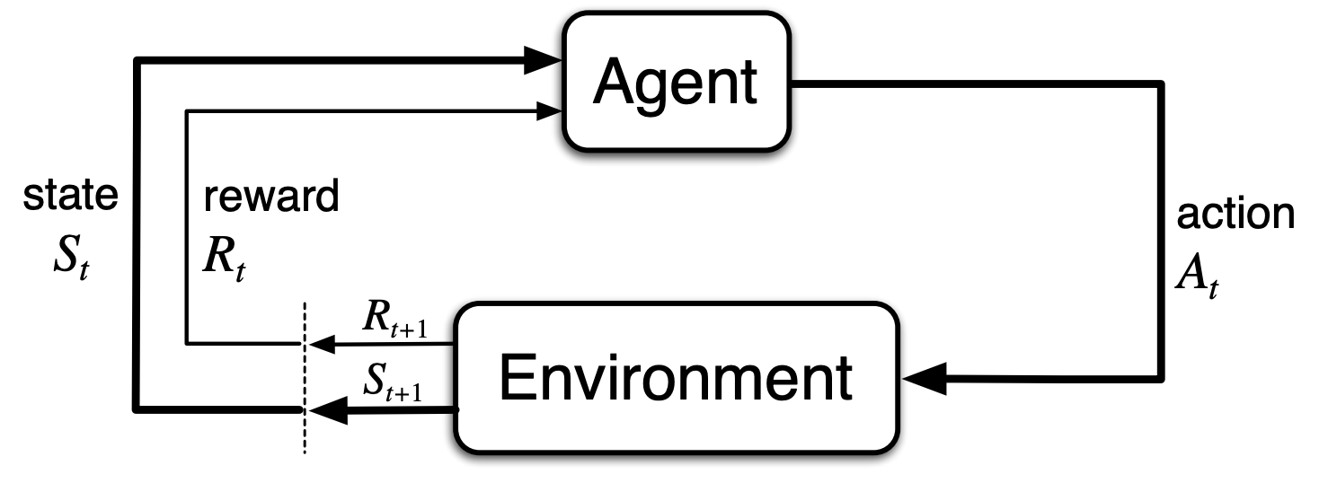
\(\pi: S_{0}, A_{0}, R_{1}, S_{1}, A_{1}, R_{2}, ... , S_{T-1}, A_{T-1}, R_{T}\)
How can we learn to act optimally without the added complexity of changing states?
A nonassociative environment is a setting that involves learning how to act in one state. A common example of a nonassociative environment is the Multi-Armed Bandit problem.
\(\pi: S, A_{0}, R_{1}, S, A_{1}, R_{2}, ... , S, A_{T-1}, R_{T}\)
This simplified setting helps us develop foundational ideas in Reinforcement Learning — like action selection and reward maximization — without worrying about state transitions.
Bandit
A bandit is a slot machine.
It is used as an analogy to represent the action an agent can make in one state.
Each action selection is like a play of one of the slot machine’s levers, and the rewards are the payoffs for hitting the jackpot, according to its underlying probability distribution.

\(\Huge{\to}\)
Rewards

Multi-Armed Bandit
A Multi-Armed Bandit can be interpreted as k-actions, or k-arms of the slot machines, to decide from.
Through repeated action selections, you maximize your winnings by concentrating actions on the best levers.


How do we decide the most appropriate action?
We calculate the expectation of a Bandit!
Each bandit has an expected reward given a particular action is selected, called the action value.
\[ Q_t(a) = \mathbb{E}[R_t | A_t = a] \]
Note that \(Q_t(a)\) tells us how good an action is at time step \(t\) for a particular action \(a\). This is fundamental concept to Value-based Reinforcement Learning algorithms.
\(Q_t(a)\) is the conditional expectation of the rewards \(R_t\) given the selection of an action \(A_t\). \(R_t\) is the random variable for the reward at time step \(t\). \(A_t\) is the random variable for the action selected at time step \(t\).
Action Value: Predicate Method
One way to compute action values is using a predicate:
\[ Q_t(a) = \frac{\sum_{i=1}^{t-1} R_i * \mathbf{1}_{A_i = a}}{\sum_{i=1}^{t-1} \mathbf{1}_{A_i = a}} \]
\(Q_t(a)\) is the action value for a particular action \(a\). \(\mathbf{1}\) is a predicate, which denotes whether \(A_i = a\) is true or false.
If the denominator is \(0\), then we denote \(Q_t(a)\) as \(0\).
Action Value: Incremental Update
To avoid computationally expensive updates using the predicate method, we can update action values in an incremental fashion:
\[ \underbrace{Q_{t+1}}_{\text{New Estimate}} = \underbrace{Q_t}_{\text{Old Estimate}} + \underbrace{\frac{1}{t}}_{\text{Step Size}} (\underbrace{R_t}_{\text{Target}} - \underbrace{Q_t}_{\text{Old Estimate}}) \]
Should we always pick actions with the highest expected value?
No, always picking actions with the highest expected value will disallow us to explore other actions!
Let’s see how we can solve this problem in the next page 😊