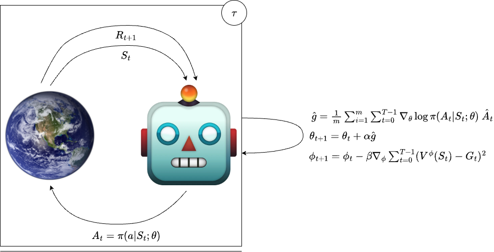
9.1 Policy Gradients
Motivation
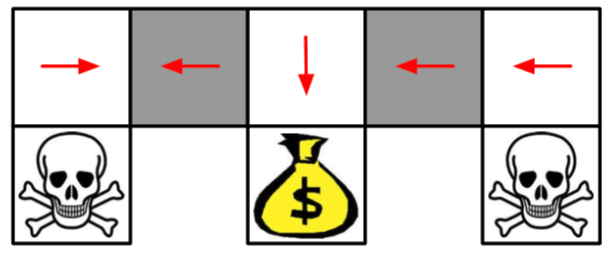
DQN is unstable and does not guarantee convergence. Following deterministic or \(\epsilon\)-greedy policies is not optimal.

Let’s learn stochastic policies using differentiable methods:
\[ \pi(a|s; \theta) \]
By following \(\pi(a|s; \theta)\), we can find optimal policy parameters \(\theta\) that maximize:
\[ V^{\pi_{\theta}}(s) = V(S_{0}; \theta) \]
Mathematical Intuition
Policy gradient algorithms search for a local maximum in \(V^{\pi_{\theta}}(s)\) using stochastic gradient ascent (SGA):
\[ \Delta \theta = \alpha \nabla V(S_{0}; \theta) \]
Ideally, we want to compute this gradient analytically.
Assume \(\pi\) is differentiable where it is non-zero:
\[ V(S_{0}; \theta) = \sum_{a} \pi(a|S_{0}; \theta) Q(S_{0},a; \theta) \]
Another formulation in terms of trajectories \(\tau\):
\[ V(S_{0}; \theta) = \sum_{\tau} P(\tau; \theta) R(\tau) \]
where \(P(\tau; \theta)\) is the probability and \(R(\tau)\) the reward of trajectory.
Using likelihood ratios:
\[ \nabla_{\theta} V(\theta) = \sum_{\tau} P(\tau; \theta) R(\tau) \nabla_{\theta} \log P(\tau; \theta) \]
Approximation using empirical estimate:
\[ \nabla_{\theta} V(\theta) \approx \hat{g} = \frac{1}{m} \sum^{m}_{i = 1} R(\tau^{i}) \nabla_{\theta} \log P(\tau^{i}; \theta) \]
Decomposing dynamics into states and actions:
\[ \nabla_{\theta} \log P(\tau^{i}; \theta) = \sum^{T-1}_{t=0} \nabla_{\theta} \log \pi(A_{t}|S_{t}, \theta) \]
This term is called the score function.
Soft-max Policy
\[ \pi(a|s;\theta) = \frac{\exp(\theta_{\text{logits}}(s)[a])}{\sum_{a'} \exp(\theta_{\text{logits}}(s)[a'])} \]
Policy Gradient Theorem
Theorem: Let \(\pi(a|s;\theta)\) be a differentiable policy. The gradient of the expected reward \(F(\theta)\) with respect to \(\theta\) is:
\[ \nabla_{\theta} F(\theta) = \mathbb{E}_{\pi_{\theta}} \left[\nabla_{\theta} \log \pi(a|s;\theta) Q^{\pi_{\theta}}(s, a)\right] \]
Addressing High Variance
Instead of multiplying the sum of rewards by the score function:
\[ \hat{g} = \frac{1}{m} \sum^{m}_{i = 1} R(\tau^{i}) \sum^{T-1}_{t=0} \log \nabla_{\theta} \pi(A_{t}|S_{t}, \theta) \]
- Use temporal structure to weight rewards relevant to each time-step:
\[ \hat{g} = \frac{1}{m} \sum^{m}_{i = 1} \sum^{T-1}_{t=0} \log \nabla_{\theta} \pi(A_{t}|S_{t}, \theta) \sum^{T-1}_{t' = t} r^{i}_{t'} \]
Baselines to Reduce Variance
Unbiased estimators \(b(s)\) help adjust for expected rewards:
\[ \hat{g} = \frac{1}{m} \sum^{m}_{i = 1} \sum^{T-1}_{t=0} \log \nabla_{\theta} \pi(A_{t}|S_{t}, \theta) (r^{i}_{t'} - b(s)) \]
Defining advantage estimates:
\[ \hat{A}_{t} = \sum^{T-1}_{t' = t} (r^{i}_{t'} - b(s)) \]
thus,
\[ \hat{g} = \frac{1}{m} \sum^{m}_{i = 1} \sum^{T-1}_{t=0} \log \nabla_{\theta} \pi(A_{t}|S_{t}, \theta) \hat{A}_{t} \]
Vanilla Policy Gradient: Illustration
Pseudocode

Exercise
Match the following concepts:
| Concept | Definition |
|---|---|
| Likelihood Ratio | \(\frac{\nabla_{\theta} \pi_{\theta}(a|s)}{\pi_{\theta}(a|s)}\) |
| Score Function | \(\nabla_{\theta} \log \pi_{\theta}(a|s)\) |
| Policy Gradient | \(\mathbb{E}_{\pi_\theta} \left[\nabla_\theta \log \pi(a|s;\theta) Q^{\pi_\theta}(s, a)\right]\) |
| Empirical Estimate | \(\frac{1}{m} \sum^{m}_{i = 1} \sum^{T-1}_{t=0} \log \nabla_\theta \pi(A_{t}|S_{t}, \theta) \hat{A}_{t}\) |
| Baseline | \(b(s)\) |