4.1 Markov Chain
A associative environment is a setting that involves learning how to act in multiple states. The best frameworks to generalize associative environments are Markov models.
Markov Models
All Markov models assume the Markov Property, meaning that future states depend only on current states and not previous states.
\[ P(s’ | s, s_{t-1}, s_{t-2}, \dots) = P(s’ | s) \]
Markov models differ based on whether every sequential state is observable and whether the system is adjusted based on observations:
| States are fully observable | States are partially observable | |
|---|---|---|
| Decision-making is not controlled | Markov Chain | Hidden Markov Model |
| Decision-making is controlled | Markov Decision Process | Partially Observable Markov Decision Process |
Markov Chain
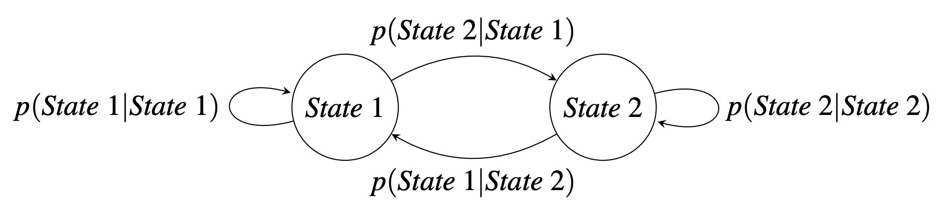
A Markov Chain is a model for transitions that are not controlled between fully observable states.
A State is a node.
A State Transition is one outward-going arrow.
State transitions are conditional probabilities of going to the next state given the current state.
Probability Matrix
Suppose a frog jumps from one lily pad to another with state transition probabilities:
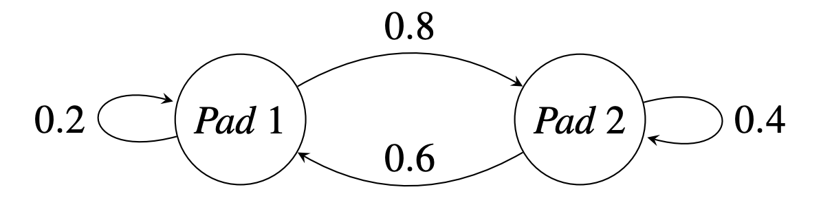
\[ \mathbf{P} = \begin{bmatrix} 0.2 & 0.6 \\ 0.8 & 0.4 \end{bmatrix} \]
Rewards Matrix
Suppose the frog has associated rewards:
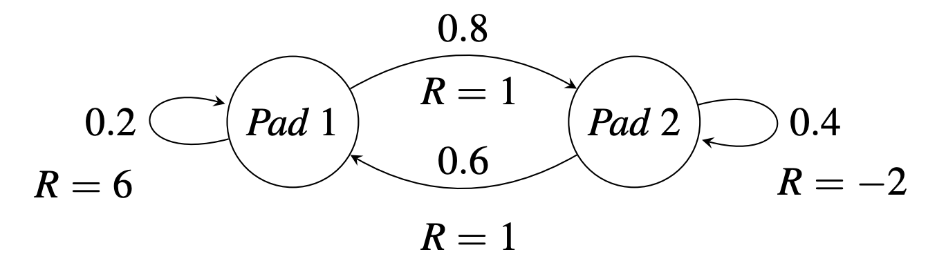
\[ \mathbf{R} = \begin{bmatrix} 6 & 1 \\ 1 & -2 \end{bmatrix} \]
Value Function
We want to calculate the expected value of moving from state \(i\) to state \(j\) for all situations \(s \in \{1,2,...,S\}\):
\[ \begin{align*} v_{j}(t) & = \sum_{i=1}^{S} p_{i,j} \ [r_{i,j}+v_{i}(t-1)] \\ & = \sum_{i=1}^{S} p_{i,j} \ r_{i,j} + \sum_{i=1}^{S} p_{i,j} \ v_{i}(t-1) \\ & = \textbf{q} + \sum_{i=1}^{S} p_{i,j}\ v_{i}(t-1) \end{align*} \]
\[ \mathbf{v}(t) = \mathbf{q} + \mathbf{v}(t-1) \mathbf{P} \]
First, we need to calculate \(\textbf{q}\), the expected reward in the next transition out of state \(i\):
\[ \mathbf{q} = \sum_{i=1}^{S} p_{i,j} r_{i,j} \]
\[ q_{1} = p_{1,1} \ r_{1,1} + r_{2,1} \ p_{2,1} \]
\[ q_{2} = p_{1,2} \ r_{1,2} + r_{2,2} \ p_{2,2} \]
\[ \textbf{q} = \begin{bmatrix} 2 & -0.2 \end{bmatrix} \]
\[ \begin{bmatrix} v_{1}(t) \ v_{2}(t) \end{bmatrix} = \begin{bmatrix} 2 \ -0.2 \end{bmatrix} + \begin{bmatrix} v_{1}(t-1) \ v_{2}(t-1) \end{bmatrix} \begin{bmatrix} 0.2 & 0.6 \\ 0.8 & 0.4 \end{bmatrix} \]
At \(t=100\): \[ \mathbf{v}(100) = \begin{bmatrix} 77.88 & 76.59 \end{bmatrix} \]
In other words, the frogs expected value at \(t = 100\) is that lilly pad \(1\) will be greater (with \(77.88\) expected flies) than that of lilly pad \(2\) (with \(76.59\) expected flies)
Asymptotic Behavior

Discounting Factor
The \(\gamma\) allows us to place a higher value on the present rewards, rather than future uncertain rewards.
\[ \mathbf{v}(t) = \mathbf{q} + \gamma \mathbf{v}(t-1) \mathbf{P} \]
\[ \begin{bmatrix} v_{1}(t) \ v_{2}(t) \end{bmatrix} = \begin{bmatrix} 2 \ -0.2 \end{bmatrix} + \gamma \begin{bmatrix} v_{1}(t-1) \ v_{2}(t-1) \end{bmatrix} \begin{bmatrix} 0.2 & 0.6 \\ 0.8 & 0.4 \end{bmatrix} \]
At \(\gamma=0.9\) and \(t=100\): \[ \mathbf{v}(100) = \begin{bmatrix} 8.47 & 7.15 \end{bmatrix} \]
Discounted Asymptotic Behavior

Python Code
import numpy as np

GAMMA = 0.9
P = np.array([[0.2, 0.6], [0.8, 0.4]])
R = np.array([[6, 1], [1, -2]])
q = np.sum(P * R, axis=1)
v_initial = np.array([0, 0])

def value_function(v, P, q, t=100):
    for _ in range(t):
        v = q + GAMMA * np.dot(v, P)
    return v

v_result = value_function(v_initial, P, q)
print(v_result)