7.1 Value Function Approximation
Motivation
Assume state \(\mathbf{s}\) is represented by a vector of continuous values.
\[ s = \begin{bmatrix} s_1 \\ s_2 \\ \vdots \\ s_n \end{bmatrix} \]
where \(s_i \in \mathbb{R}\) for all \(i = 1, 2, \ldots, n\)
\(\because s\) is the representation of any state information.
Tabular representation for \(s_i\) does not work now. What if the interval for \(s_i\) is infinite?
Develop a function with parameters \(\mathbf{w}\) that approximates the value of these continuous state values:
\[ \hat{V}(s; \mathbf{w}) \approx V_{\pi}(s) \]
Now, we can generalize approximate values of states encountered and those we have not.
Types of Value Function Approximators
There are many ways of constructing \(\hat{V}(s; \mathbf{w})\):
- Ensemble methods (decision trees, nearest neighbors, etc.)
- Fourier basis
- Much more…
We will focus only on differentiable methods:
- Linear combination of features (today’s lecture)
- Neural networks (next lecture: DQN)
The purpose is to update our parameters \(\mathbf{w}\) using mean-squared error (MSE) and stochastic gradient descent (SGD).
Updating Value Function Approximators
Recall MSE for supervised learning:
\[ F(\mathbf{x}_{k}) = \mathbb{E}[(\mathbf{t}_{k} - \mathbf{a}_{k})^2] \]
Recall SGD for supervised learning:
\[ \mathbf{x}_{k+1} = \mathbf{x}_{k} - \alpha \nabla_{\mathbf{x}_{k}} F(\mathbf{x}_{k}) \]
Optimizing Value Function Approximators
Our loss function will optimize for our parameter vector \(\mathbf{w}\) while minimizing MSE between our approximate value \(\hat{V}(s; \mathbf{w})\) and our “true value” \(V_{\pi}(s)\):
\[ F(\mathbf{w}_{t}) = \mathbb{E}_{\pi}[(V_{\pi}(S_{t}) - \hat{V}(S_{t}; \mathbf{w}_{t}))^{2}] \]
SGD update for parameters \(\mathbf{w}\):
\[ \mathbf{w}_{t+1} = \mathbf{w}_{t} + \alpha(V_{\pi}(S_{t}) - \hat{V}(S_{t}; \mathbf{w}_{t}))\nabla_{\mathbf{w}_{t}} \hat{V}(S_{t}; \mathbf{w}_{t}) \]
Derivative of MSE loss:
\[ \nabla_{\mathbf{w}_{t}} F(\mathbf{w}_{t}) \approx -2(V_{\pi}(S_{t}) - \hat{V}(S_{t}; \mathbf{w}_{t}))\nabla_{\mathbf{w}_{t}} \hat{V}(S_{t}; \mathbf{w}_{t}) \]
Plug derivative of MSE loss into SGD equation:
\[ \begin{align} \mathbf{w}_{t+1} &= \mathbf{w}_{t} - \alpha \nabla_{\mathbf{w}_{t}} F(\mathbf{w}_{t}) \\[10pt] &= \mathbf{w}_{t} - \alpha (-2(V_{\pi}(S_{t}) - \hat{V}(S_{t}; \mathbf{w}_{t}))\nabla_{\mathbf{w}_{t}} \hat{V}(S_{t}; \mathbf{w}_{t})) \\[10pt] &= \mathbf{w}_{t} + 2\alpha(V_{\pi}(S_{t}) - \hat{V}(S_{t}; \mathbf{w}_{t}))\nabla_{\mathbf{w}_{t}} \hat{V}(S_{t}; \mathbf{w}_{t}) \\[10pt] &= \mathbf{w}_{t} + \alpha(V_{\pi}(S_{t}) - \hat{V}(S_{t}; \mathbf{w}_{t}))\nabla_{\mathbf{w}_{t}} \hat{V}(S_{t}; \mathbf{w}_{t}) \end{align} \]
Feature Representations
Prior to calculating \(\hat{V}(s; \mathbf{w})\), we must preprocess \(\mathbf{s}\) to construct proper feature representations:
\[ \mathbf{f}(s) = \begin{bmatrix} s_1 \\ s_2 \\ \vdots \\ s_d \end{bmatrix} \]
Some types of feature representations \(\mathbf{f}\) include:
- One-hot encoding
- Polynomials
- Radial basis functions
- State normalization (homework)
- Tile coding (homework)
State normalization ensures consistent scaling between \(0\) and \(1\):
\[ \mathbf{f}(s) = \begin{bmatrix} \frac{s_1 - \text{lower bound}_{1}}{\text{upper bound}_{1} - \text{lower bound}_{1}} \\ \frac{s_2 - \text{lower bound}_{2}}{\text{upper bound}_{2} - \text{lower bound}_{2}} \\ \vdots \\ \frac{s_d - \text{lower bound}_{d}}{\text{upper bound}_{d} - \text{lower bound}_{d}} \end{bmatrix} \]
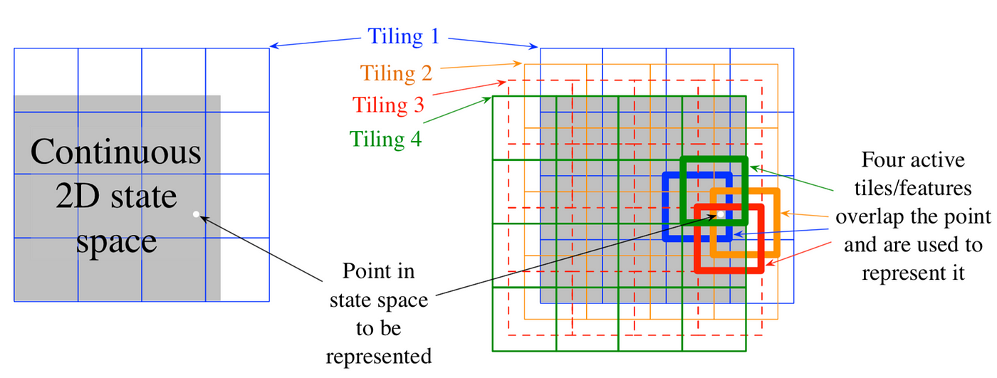
Tile coding is a one-hot representation for multi-dimensional continuous spaces that is flexible and computationally efficient.
\[ \mathbf{f}(s) = \begin{bmatrix} \delta(s, T_1) \\ \delta(s, T_2) \\ \vdots \\ \delta(s, T_d) \end{bmatrix} \text{where} \ d \ \text{is the number of tilings} \]
\[ \delta(s, T_i) = \begin{cases} 1 & \text{if } s \in T_i \\ 0 & \text{otherwise} \end{cases} \]
Exercise
Based on your mathematical intuition using SGD, are we guaranteed convergence to a local or global minimum?
\[ \mathbf{w}_{t+1} = \mathbf{w}_{t} + \alpha(V_{\pi}(S_{t}) - \hat{V}(S_{t}; \mathbf{w}_{t}))\nabla_{\mathbf{w}_{t}} \hat{V}(S_{t}; \mathbf{w}_{t}) \]