4.2 Markov Decision Process (MDP)
Markov Chain’s are a framework for an associative environment.
A Markov Chain is a model for transitions that are not controlled between fully observable states.
Ideally, we would like to have an Agent that can control state transitions in any associative environment.
How can we learn to act optimally with changing states but controlling state transitions between fully observable states?
We need to model our environments as a Markov Decision Process (MDP).
| States are fully observable | States are partially observable | |
|---|---|---|
| Decision-making is not controlled | Markov Chain (MC) | Hidden Markov Model (HMM) |
| Decision-making is controlled | Markov Decision Process (MDP) | Partially Observable Markov Decision Process (POMDP) |
Markov Decision Process
A Markov Decision Process (MDP) is a model for transitions that are controlled between fully observable states.
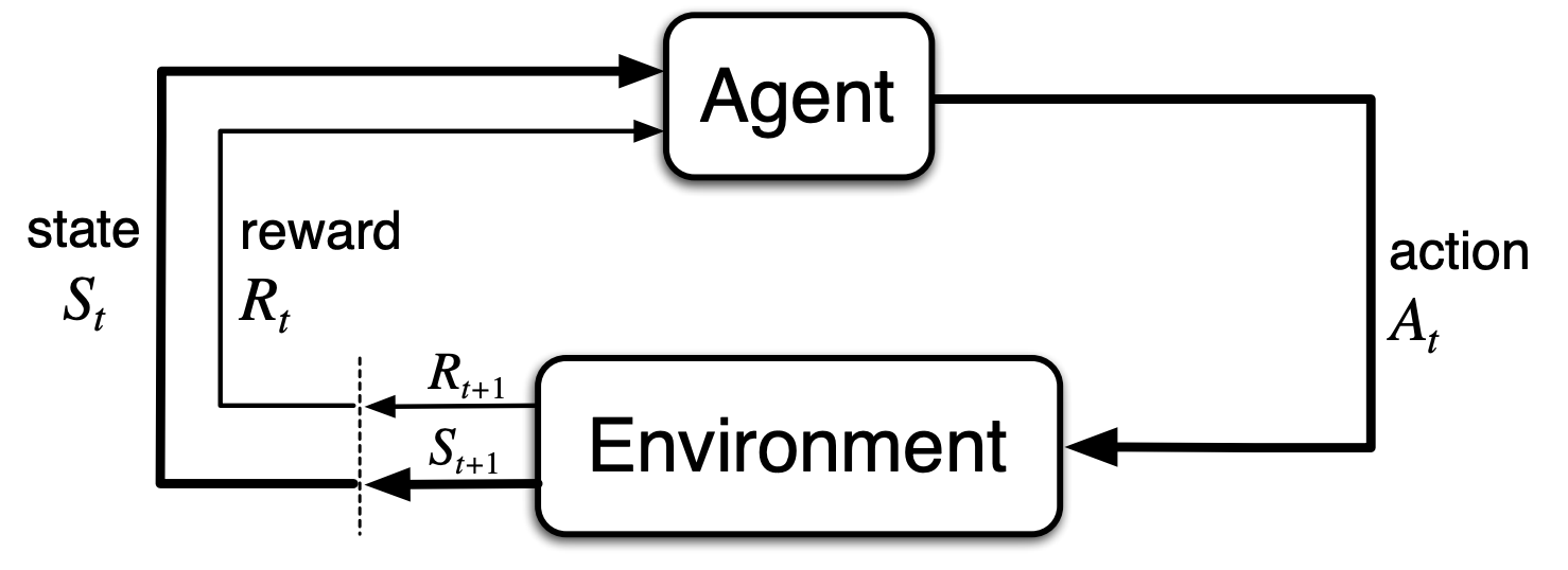
The Agent is the learner and decision-maker.
The Environment is everything external to the agent.
From an Initial State, the agent interacts with the environment through its Actions.
These actions continuously give rise to different States and Rewards.
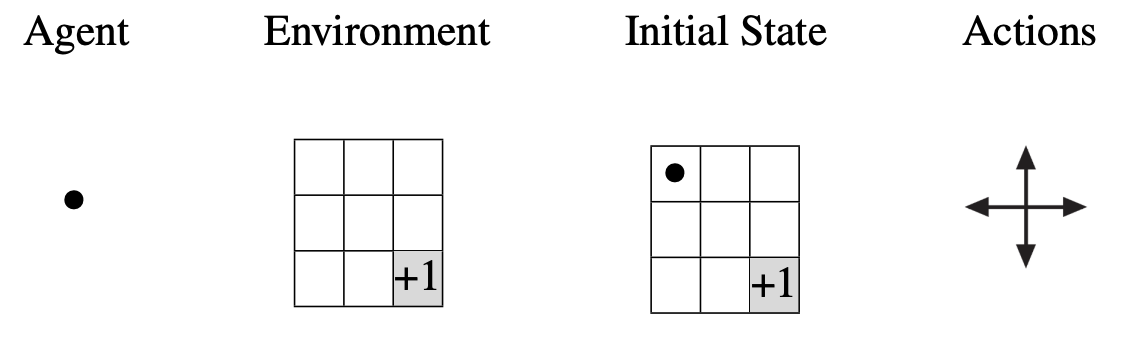
- Actions are equally likely to occur.
- Actions that take the agent out of the environment receive a reward of \(-1\), actions that take the agent to the terminal state (shaded in gray) receive a reward of \(+1\), and all other actions receive a reward of \(0\).
- Our objective is to calculate the shortest path from any state to the optimal state.
Sequential Interaction
For a finite discrete number of time steps \(t = 0, 1, 2, 3...,T\) (where \(T\) is the terminal time step marking the end of an episode) the sequential interaction is:
- The agent receives an interpretation from the state \(s_t \in S\).
- The agent makes an action \(a_t \in A(s_t)\) based on the situation.
- The agent receives a reward \(r_{t+1} \in R \subseteq \mathbb{R}\) from its environment and finds itself in a new state \(s_{t+1}\) based on the action taken.
The sequence continues in the form:
\[ s_0, a_0, r_1, s_1, a_1, r_2, s_2, a_2, r_3,... \]
Sequential interaction for one episode:
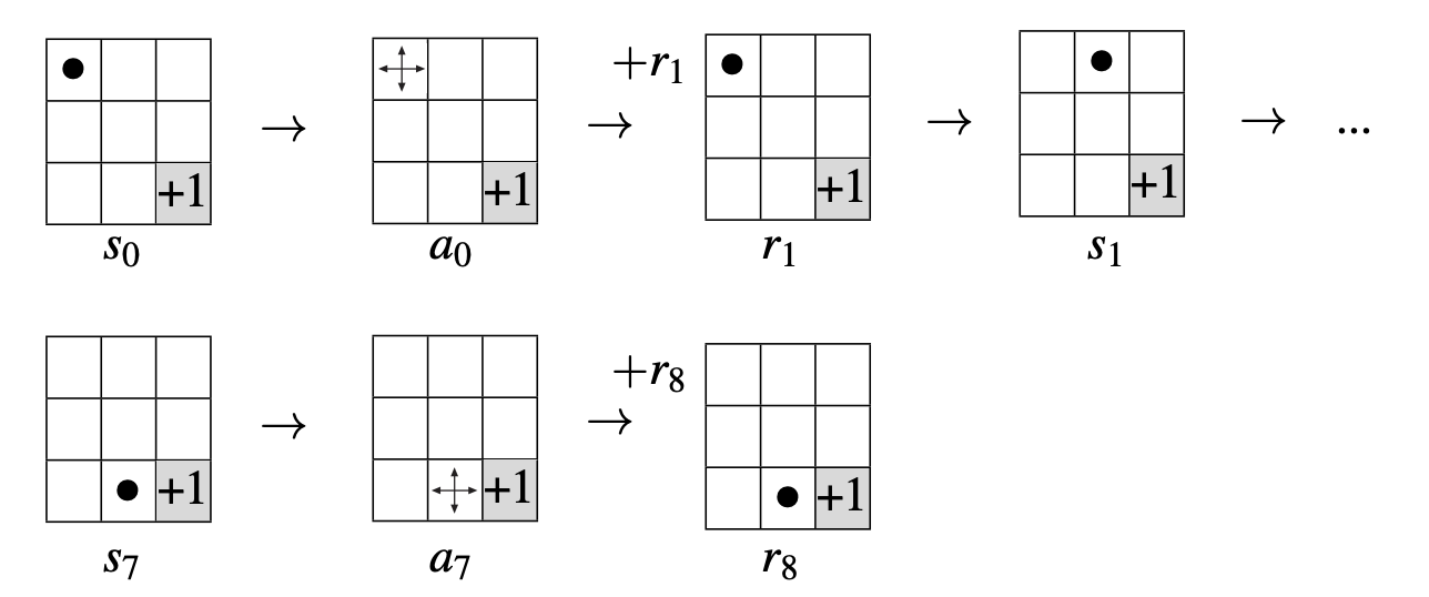
Notice that, for now, state transitions are deterministic. In other words, we assume a perfect model of the environment. We do not care about stochastic state transitions (this is something that we will visit in the next lectures).
Policy
A Policy is a mapping from states to probabilities of selecting each possible action, denoted as:
\[ \pi(a|s) \]
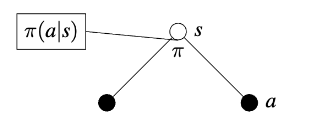
\[ \sum_{a \in A(s)} \pi(a|s) = 1 \quad \text{for all } s \in S \]
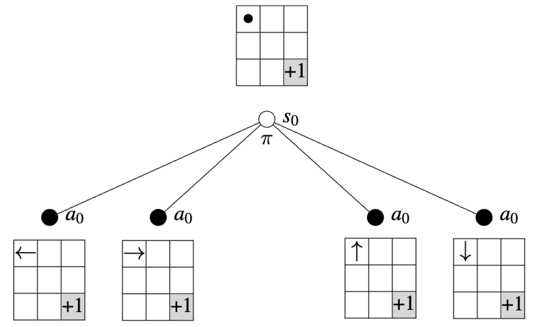
Since all actions are equally likely, we are said to be following a random policy:
\[ \pi(a_0|s_0) = \frac{1}{4} \]
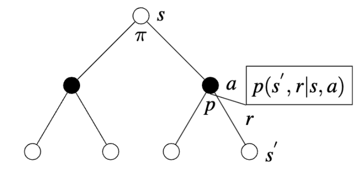
Dynamic Function
The dynamic function is a mapping of the state transition probabilities of the MDP for each possible reward:
\[ p(s^{'}, r | s, a) \]
As mentioned before, the dynamics of GridWorld are deterministic leading to the same new state given each state and action:
\[ \sum_{s^{'} \in S}\sum_{r \in R} p(s^{'}, r| s, a) = 1 \quad \text{for all } s \in S \text{ and } a \in A(s) \]
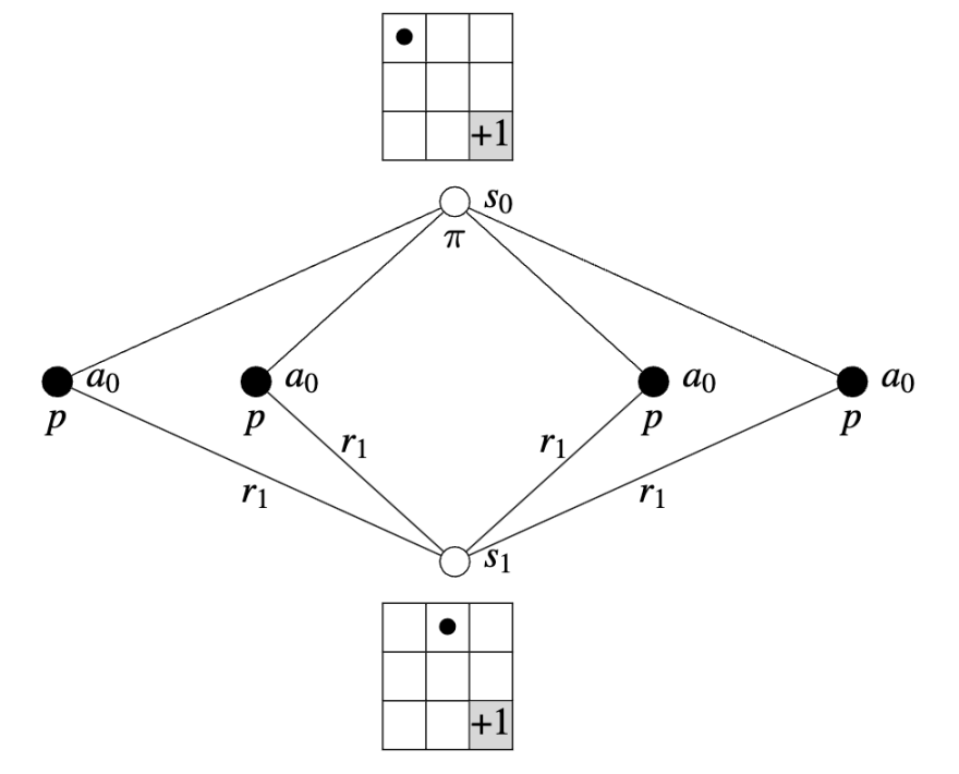
As mentioned before, the dynamics of GridWorld are deterministic, leading to the same new state given each state and action:
\[ p(s_{1}, r_{1}| s_0, a_{0}) = 1 \]
Goal
Our Goal \(G_{t}\) is to maximize the expected return of the discounted reward sequence:
\[ \begin{aligned} G_{t} = r_{t+1} + \gamma r_{t+2} + \ldots + \gamma^{T-1} r_{T} \\ = r_{t+1} + \gamma (r_{t+2} + \ldots + \gamma^{T-2} r_{T}) \\ = r_{t+1} + \gamma G_{t+1} \end{aligned} \]
Suppose \(\gamma = 0.5\) and the following sequence of rewards is received \(r_{1} = -1\), \(r_{2} = 2\), \(r_{3} = 6\), \(r_{4} = 3\), and \(r_{5} = 2\), with \(T = 5\). What are \(G_{0}\), \(G_{1}\), …, \(G_{5}\)?
\[ \begin{aligned} G_{5} &= r_{6} + r_{7} + \dots = 0 \\ G_{4} &= r_{5} + 0.5(G_{5}) = 2 \\ G_{3} &= r_{4} + 0.5(G_{4}) = 4 \\ G_{2} &= r_{3} + 0.5(G_{3}) = 8 \\ G_{1} &= r_{2} + 0.5(G_{2}) = 6 \\ G_{0} &= r_{1} + 0.5(G_{1}) = 2 \\ \end{aligned} \]
Value Functions
Value Functions calculate the expected reward when starting from the state \(s\) and then interacting with the environment according to the policy \(\pi\), denoted as:
\[ v_{\pi}(s) = \mathbb{E_{\pi}}[G_{t}| \ s] \]
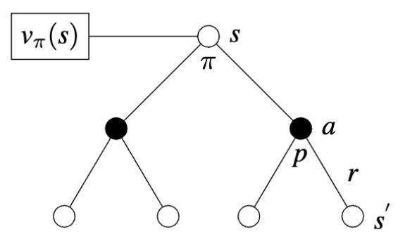
Bellman Equation
For any policy \(\pi\) and any state \(s\), the Bellman equation holds:
\[ \begin{aligned} v_{\pi}(s) &= \mathbb{E_{\pi}}[G_{t}| \ s] \\ &= \mathbb{E_{\pi}}[r_{t+1} + \gamma G_{t+1}| \ s] \\ &= \sum_{a} \pi(a|s) \sum_{s^{'},r} p(s^{'},r|s,a)[r_{t+1} + \gamma \mathbb{E_{\pi}}[G_{t+1}| \ s]] \\ &= \underbrace{\sum_{a} \pi(a|s)}_{Policy} \underbrace{\sum_{s^{'}, r} p(s^{'},r|s,a)}_{Dynamic \ Function}\underbrace{[r_{t+1} + \gamma v_{\pi}(s^{'})]}_{Discounted \ Reward \ Sequence} \end{aligned} \]
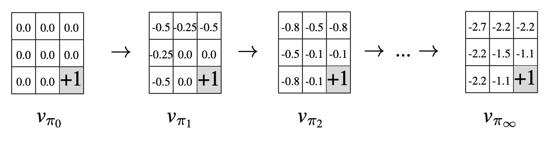
For the first episode, calculate the value of each state using the Bellman equation:
\[ v_{\pi}(s) = \sum_{a} \pi(a|s) \sum_{s^{'}, r} p(s^{'},r|s,a)[r + \gamma v_{\pi}(s^{'})] \]
![]()
Action Value Functions
Action Value Functions estimate how good it is for an agent to follow policy \(\pi\) given the action taken under the previous state:
\[ q_{\pi}(s, a) = \mathbb{E_{\pi}}[G_{t}| \ s, \ a] \]
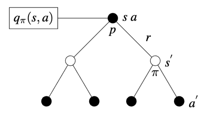
Bellman Equation
The action value function is also expressed in terms of the Bellman equation:
\[ \begin{align} q_{\pi}(s, a) & = \mathbb{E_{\pi}}[G_{t}| \ s, \ a] \\ & = \underbrace{\sum_{s^{'}, r} p(s^{'},r|s,a)}_{Dynamic \ Function} \underbrace{[r + \gamma v_{\pi}(s^{'})]}_{Discounted \ Reward \ Sequence} \end{align} \]
Notice that the policy is no longer calculated (since an action has already taken place according to the policy), and that the quality of following policy \(\pi\) is calculated in \(v_{\pi}(s^{'})\).
Optimal Policy
An optimal policy \(\pi\) is defined to be better than or equal to a policy \(\pi^{'}\) if its expected return is greater than or equal to that of \(\pi^{'}\) for all states:
\[ \pi \geq \pi^{'} \quad \text{I.F.F.} \quad v_{\pi} \geq v_{\pi^{'}} \quad \forall s \in S \]
Since there may be more than one optimal policy, we denote all optimal policies by \(\pi_{*}\).
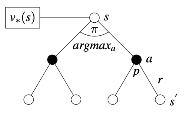
Optimal Value Function
\[ v_{*}(s) = \max_{a} \sum_{s^{'}, r} p(s^{'},r|s,a) \big[ r + \gamma v_{*}(s^{'}) \big] \]
Optimal Action-Value Function
\[ q_{*}(s, a) = \sum_{s^{'}, r} p(s^{'},r|s,a) \big[ r + \gamma v_{*}(s^{'}) \big] \]
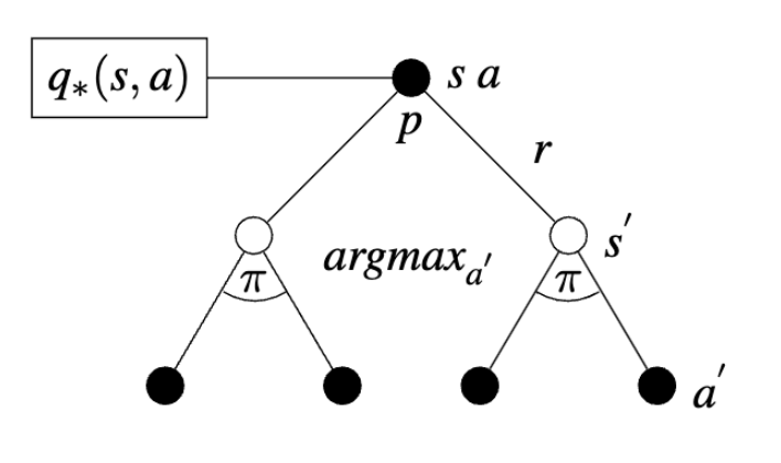
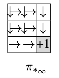
For the first episode, calculate the optimal value for each state using the bellman equation:
\[ v_{*}(s) = \max_{a} \sum_{s^{'}, r} p(s^{'},r|s,a) \big[ r + \gamma v_{*}(s^{'}) \big] \]
![]()
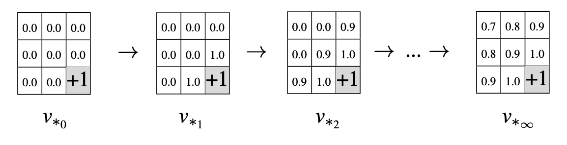
Notice the behavior of the optimal policy as \(\pi_{*} \to \infty\)