7.1 Value Function Approximation
Assume state \(\mathbf{s}\) is represented by a vector of continuous values.
\[ \mathbf{s} = \begin{bmatrix} s_1 \\ s_2 \\ \vdots \\ s_n \end{bmatrix} \]
where \(s_i \in \mathbb{R}\) for all \(i = 1, 2, \ldots, n\)
Tabular representation for \(s_i\) does not work now. What if the interval for \(s_i\) is infinite?
Consider the following OpenAI Gymnasium MountainCar environment (Moore 1990):
The state information \(\mathbf{s}\) is now the following vector:
\[ \mathbf{s} = \begin{bmatrix} p \in (-1.2,0.6) \gets \text{position of the car along the x-axis} \\ v \in (-0.07,0.07) \gets \text{velocity of the car} \\ \end{bmatrix} \]
The environment has a discrete action space \(\mathcal{A}\):
\[ \mathcal{A} = \{0 \gets \text{Accelerate to the left},1 \gets \text{Don’t accelerate},2 \gets \text{Accelerate to the right}\} \]
The environments state transition dynamics \(P(s',r|s,a)\) are :
\[ v_{t+1} = v_t + (A_t - 1) * \underbrace{0.001}_{\text{force}} - cos(3 * p_t) * \underbrace{0.0025}_{\text{gravity}} \] \[ p_{t+1} = p_t + v_{t+1} \]
The goal is to reach the flag placed on top of the right hill as quickly as possible, as such the agent is penalised with a reward \(R\) of \(-1\) for each timestep.
The episode ends \(d\) (dones) if either of the following happens:
- Termination: The position \(p\) of the car is greater than or equal to \(0.5\) (the goal position on top of the right hill)
- Truncation: The length of the episode is \(200\).
Types of Value Function Approximators
There are many ways of constructing \(\hat{V}(s; \mathbf{w})\):
- Ensemble methods (decision trees, nearest neighbors, etc.)
- Fourier basis
- Much more…
We will focus only on differentiable methods:
- Linear combination of features (today’s lecture)
- Neural networks (next lecture: DQN)
The purpose is to update our parameters \(\mathbf{w}\) using mean-squared error (MSE) and stochastic gradient descent (SGD).
Updating Value Function Approximators
Our loss function will optimize for our parameter vector \(\mathbf{w}\) while minimizing MSE between our approximate value \(\hat{V}(s; \mathbf{w})\) and our “true value” \(V_{\pi}(s)\):
\[ F(\mathbf{w}_{t}) = \mathbb{E}_{\pi}[(V_{\pi}(S_{t}) - \hat{V}(S_{t}; \mathbf{w}_{t}))^{2}] \]
Recall Mean Squared Error (MSE) for supervised learning:
\[ F(\mathbf{x}_{k}) = \mathbb{E}[(\mathbf{t}_{k} - \mathbf{a}_{k})^2] \]
Recall Stochastic Gradient Descent (SGD) for supervised learning:
\[ \mathbf{x}_{k+1} = \mathbf{x}_{k} - \alpha \nabla_{\mathbf{x}_{k}} F(\mathbf{x}_{k}) \]
SGD update for parameters \(\mathbf{w}\):
\[ \mathbf{w}_{t+1} = \mathbf{w}_{t} + \alpha(V_{\pi}(S_{t}) - \hat{V}(S_{t}; \mathbf{w}_{t}))\nabla_{\mathbf{w}_{t}} \hat{V}(S_{t}; \mathbf{w}_{t}) \]
Plug derivative of MSE loss into SGD equation:
\[ \begin{align} \mathbf{w}_{t+1} &= \mathbf{w}_{t} - \alpha \nabla_{\mathbf{w}_{t}} F(\mathbf{w}_{t}) \\[10pt] &= \mathbf{w}_{t} - \alpha (-2(V_{\pi}(S_{t}) - \hat{V}(S_{t}; \mathbf{w}_{t}))\nabla_{\mathbf{w}_{t}} \hat{V}(S_{t}; \mathbf{w}_{t})) \\[10pt] &= \mathbf{w}_{t} + 2\alpha(V_{\pi}(S_{t}) - \hat{V}(S_{t}; \mathbf{w}_{t}))\nabla_{\mathbf{w}_{t}} \hat{V}(S_{t}; \mathbf{w}_{t}) \\[10pt] &= \mathbf{w}_{t} + \alpha(V_{\pi}(S_{t}) - \hat{V}(S_{t}; \mathbf{w}_{t}))\nabla_{\mathbf{w}_{t}} \hat{V}(S_{t}; \mathbf{w}_{t}) \end{align} \]
State Preprocessing
Prior to calculating \(\hat{V}(s; \mathbf{w})\), we must preprocess \(\mathbf{s}\) to construct proper feature representations:
\[ \mathbf{f}(s) = \begin{bmatrix} s_1 \\ s_2 \\ \vdots \\ s_d \end{bmatrix} \]
Some types of feature representations \(\mathbf{f}\) include:
- One-hot encoding
- Polynomials
- Radial basis functions
- State normalization (homework)
- Tile coding (homework)
State normalization ensures consistent scaling between \(0\) and \(1\):
\[ \mathbf{f}(s) = \begin{bmatrix} \frac{s_1 - \text{lower bound}_{1}}{\text{upper bound}_{1} - \text{lower bound}_{1}} \\ \frac{s_2 - \text{lower bound}_{2}}{\text{upper bound}_{2} - \text{lower bound}_{2}} \\ \vdots \\ \frac{s_d - \text{lower bound}_{d}}{\text{upper bound}_{d} - \text{lower bound}_{d}} \end{bmatrix} \]
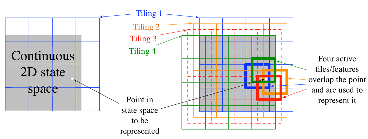
Tile coding is a one-hot representation for multi-dimensional continuous spaces that is flexible and computationally efficient.
\[ \mathbf{f}(s) = \begin{bmatrix} \delta(s, T_1) \\ \delta(s, T_2) \\ \vdots \\ \delta(s, T_d) \end{bmatrix} \text{where} \ d \ \text{is the number of tilings} \]
\[ \delta(s, T_i) = \begin{cases} 1 & \text{if } s \in T_i \\ 0 & \text{otherwise} \end{cases} \]
Based on your mathematical intuition using SGD, are we guaranteed convergence to a local or global minimum?
\[ \mathbf{w}_{t+1} = \mathbf{w}_{t} + \alpha(V_{\pi}(S_{t}) - \hat{V}(S_{t}; \mathbf{w}_{t}))\nabla_{\mathbf{w}_{t}} \hat{V}(S_{t}; \mathbf{w}_{t}) \]
Hint: Think about Lecture 1